Biology For Dummies
Part III It’s a Small, Interconnected World
Chapter 11
Observing How Organisms Get Along
In This Chapter
Discovering how organisms interact with each other and their environment
Analyzing populations and their growth (or lack thereof)
Tracing the path of energy and matter on planet Earth
One of the amazing things about this planet is that even though different parts of the world have different climates, the organisms living there somehow manage to get what they need to survive from each other and the world around them. This chapter explores Earth’s various ecosystems and details how the interactions between organisms work to keep life on Earth in balance. It also covers how scientists study groups of organisms to stay on top of how their populations are growing (or declining).
Ecosystems Bring It All Together
Life thrives in every environment on Earth, and each of those environments is its own ecosystem, a group of living and nonliving things that interact with each other in a particular environment. An ecosystem is essentially a little machine made up of living and nonliving parts. The living parts, called biotic factors, are all the organisms that live in the area. The nonliving parts, called abiotic factors, are the nonliving things in the area (think air, sunlight, and soil).
Ecosystems exist in the world’s oceans, rivers, forests — they even exist in your backyard and local park. They can be as huge as the Amazon rain forest or as small as a rotting log. The catch is that the larger an ecosystem is, the greater the number of smaller ecosystems existing within it. For example, the ecosystem of the Amazon rain forest also consists of the soil ecosystem and the cloud forest ecosystem (found at the tops of the trees).
 A particular branch of science called ecology is devoted to the study of ecosystems, specifically how organisms interact with each other and their environment. Scientists who work in this branch are called ecologists, and they look at the interactions between living things and their environment on many different scales, from large to small.
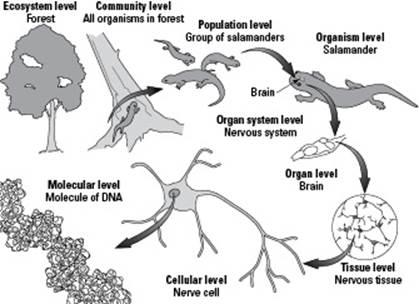
The sections that follow explain how ecologists classify Earth’s various ecosystems and how they describe the interactions between the planet’s many species. Before you check them out, take a look at Figure 11-1 to get an idea of how living things are organized.
Figure 11-1: The organization of living things.
Biomes: Communities of life
All the living things together in an ecosystem form a community. For example, a forest community may contain trees, shrubs, wildflowers, squirrels, birds, bats, insects, mushrooms, bacteria, and much more. The different types of communities found on Earth are called biomes. Six major types of biomes exist:
Freshwater biomes include ponds, rivers, streams, lakes, and wetlands. Only about 3 percent of the Earth’s surface is made up of freshwater, but freshwater biomes are home to many different species, including plants, algae, fish, and insects. Wetlands, in particular, have the greatest amount of diversity of any of the biomes.
Marine biomes contain saltwater and include the oceans, coral reefs, and estuaries. They cover 75 percent of the Earth’s surface and are very important to the planet’s oxygen and food supply — more than half the photosynthesis that occurs on Earth occurs in the ocean (we describe the process of photosynthesis in Chapter 5). Marine biomes are home to many marine creatures such as algae, fish, octopuses, dolphins, and whales.
 Estuaries are areas where saltwater mingles with freshwater. They include familiar places such as bays, sounds, lagoons, salt marshes, and beaches. Estuaries are an important habitat for many different species, including birds, fish, and shellfish. Because they provide a habitat for young fish, estuaries are vital to the health of commercial fisheries. Unfortunately, estuaries are typically found on the coast, which is also prime real estate for people. As a result, estuaries are being heavily impacted by human development.
Desert biomes receive minimal amounts of rainfall and cover approximately 20 percent of the Earth’s surface. Plants and animals that live in deserts have special adaptations, such as the ability to store water or only grow during the rainy season, to help them survive in the low-water environment. Some familiar desert inhabitants are cacti, reptiles, birds, camels, rabbits, and dingoes.
Forest biomes contain many trees or other woody vegetation; cover about 30 percent of the Earth’s surface; and are home to many different plants and animals, including trees, skunks, squirrels, wolves, bears, birds, and wildcats. They’re important for global carbon balance because they pull carbon dioxide out of the atmosphere through the process of photosynthesis. Forests are being heavily impacted by human development as humans seek additional land for homes and agriculture and cut down forests for their wood.
Rain forests are evergreen forests that receive lots of rainfall and are incredibly rich in species diversity. As many as half the world’s animals live in rain forests, including gorillas, tree frogs, butterflies, tigers, parrots, and boa constrictors.
Grassland biomes are dominated by grasses, but they’re also home to many other species, such as birds, zebras, giraffes, lions, buffaloes, termites, and hyenas. Grasslands cover about 30 percent of the Earth’s surface and are typically flat, have few trees, and possess rich soil. Because of these features, people converted many natural grasslands for agricultural purposes.
Tundra biomes are very cold and have very little liquid water. Tundras cover about 15 percent of the planet’s surface and are found at the poles of the Earth as well as at high elevations. Arctic tundras are home to organisms such as arctic foxes, caribou, and polar bears, whereas mountain tundras are home to mountain goats, elk, and birds. In both types of tundra, nutrients are typically scarce, and the growing seasons are quite short.
Why can’t we be friends: Interactions between species
Not all the organisms in a given community are the same. In fact, they’re often members of different species (meaning they can’t sexually reproduce together). Yet these organisms must interact with each other as they go about their daily business of finding what they need to survive. Of course, just like relationships between people, relationships between other species can be good, bad, or just so-so.
Ecologists use a few specific terms to describe the types of interactions between different species:
Mutualism: Both organisms benefit in a mutualistic relationship. Case in point: You give the bacteria in your small intestines a nice place to live complete with lots of food, and they make vitamins for you. Another example is when fungi in the soil form partnerships with plant roots. The fungi, called mycorrhizae, grow on the plant roots and help the roots absorb water and minerals from a wider area within the soil. In return, the mycorrhizae get some sugar from the plant.
Competition: Both organisms suffer in a competitive relationship. If a resource such as food, space, or water, is in limited supply, species struggle with each other to obtain enough to survive. Just think of a vegetable garden that’s overrun with weeds. In this scenario, the vegetable plants can’t do well because they’re competing with the weeds for water, minerals, and space. As a result, all the plants grow smaller and weaker in the crowded space than they would if they were growing by themselves.
Predation and parasitism: One organism benefits at the expense of the other in predatory and parasitic relationships. When a lion eats a gazelle, the benefits are purely the lion’s. Likewise, when a dog gets worms, the worms have a happy home and lots of food, but the dog doesn’t get enough nutrition. The only real difference between these two situations is the speed of the interaction. In predation, one organism kills and eats the other right away; in parasitism, one organism slowly feeds off the other.
Studying Populations Is Popular in Ecology
Each group of organisms of the same species living in the same area forms a population. For instance, the forests in the Pacific Northwest consist of Douglas fir trees and Western red cedars. Because Doug firs and Western red cedars are two different kinds of trees, ecologists consider two groups of these trees in the same forest to be two different populations.
Population ecology is the branch of ecology that studies the structures of populations and how they change. (Population biology is a very similar field that also includes the study of the genetics of populations.)
The following sections introduce you to some of the basic concepts of population ecology. They also help you understand the ways in which populations grow and change, as well as how scientists measure and study their growth, and give you some insight into the massive growth of the human population.
Reviewing the basic concepts of population ecology
Like all ecologists, population ecologists are interested in the interactions of organisms with each other and with their environment. The unique thing about population ecologists, though, is that they study these relationships by examining the properties of populations rather than individuals.
The next few sections walk you through some of the basic properties of populations and show you why they’re important.
Population density
One way of looking at the structure of a population is in terms of its population density (how many organisms occupy a specific area).
Say you want to get an idea of how the human population is distributed in the state of New York. About 19.5 million people live in the 47,214 square miles that make up the state. If you divide the number of people by the area, you get a population density of about 413 people per square mile. However, the human population of New York isn’t evenly distributed. In order to really understand how the human population is distributed in the state of New York, you need to compare the population density of the state to the population density of New York City.
The New York City metropolitan area has 8,214,426 people living in just 303 square miles, creating a population density of 27,110 people per square mile. If all the people in New York City were evenly distributed, each person would have 1 1/2 acres of space all to herself (there are 640 acres in 1 square mile). However, people living in New York City actually have only 3/10 of an acre, which is only 1,300 square feet, to themselves.
All of these numbers just go to show that the human population in New York is heavily concentrated in New York City and much less concentrated in other areas of the state.
Dispersion
Population ecologists use the term dispersion to describe the distribution of a population throughout a certain area. Populations disperse in three main ways:
Clumped dispersion: In this type of dispersion, most organisms are clustered together with few organisms in between. Examples include people in New York City, bees in a hive, and ants in a hill.
Uniform dispersion: Uniformly dispersed organisms are spread evenly throughout an area. Grapevines in a vineyard and rows of corn plants in a field are examples of uniform dispersion.
Random dispersion: In this type of dispersion, one place in the area is as good as any other for finding the organism. (Note: Random dispersion is rare in nature but may result when seeds or larvae are scattered by wind or water.) Examples of random dispersion include barnacles scattered on the surfaces of rocks and plants with wind-blown seeds settling down on bare ground.
Population dynamics
Population dynamics are changes in population density over time or in a particular area. Population ecologists typically use age-structure diagrams to study these changes and note trends.
Age-structure diagrams, sometimes called population pyramids, show the numbers of people in each age group in a population at a particular time. The shape of an age-structure diagram can tell you how fast a population is growing.
A pyramid-shaped age-structure diagram indicates the population is growing rapidly. Take a look at Figure 11-2a. In Mexico, more people are below reproductive age than above reproductive age, giving the age-structure diagram a wide base and a narrow top. The newest generations are larger than the generations before them, so the population size is increasing.
An evenly shaped age-structure diagram indicates the population is relatively stable. According to Figure 11-2b, the number of people above and below reproductive age in Iceland is about equal, with a decrease in the population as the older group ages. The newest generations are about the same size as the generations before them, so the population is staying roughly the same size.
An age-structure diagram that has a smaller base than middle portion indicates the population is decreasing in size. When you refer to Figure 11-2c, you notice that more people are above reproductive age in Japan than below it. The newest generations are smaller than the older generations, so the population is decreasing.
Survivorship
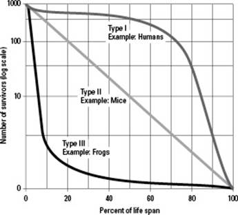
Scientists interested in demography — the study of birth, death, and movement rates that cause change in populations — noticed that different types of organisms have distinct patterns in how long offspring survive after birth. The scientists followed groups of organisms that were all born at the same time and looked at their survivorship, which is the number of organisms in the group that are still alive at different times after birth. They then plotted out survivorship curves, graphs that plot survival after birth over time (like the one in Figure 11-3), to depict how long individuals typically survive in a population.
Three types of survivorship exist:
Type I survivorship: Most offspring survive, and organisms live out most of their life span, dying in old age. Humans have a Type I survivorship because most individuals survive to middle age (about 40 years) and beyond.
Type II survivorship: Death occurs randomly throughout the life span, usually due to predation or disease. Mice have Type II survivorship — they never know when the cat or mousetrap will strike.
Type III survivorship: Most organisms die young, and few members of the population survive to reproductive age. However, individuals that do survive to reproductive age often live out the rest of their life span and die in old age. In other words, Type III organisms die young. Species such as frogs that produce offspring that must swim on their own as larvae fit into this category. Other animals eat many of the larvae before they reach the adult stage (which is when they can reproduce).
Figure 11-2:Age-structure diagrams break down age groups in populations.
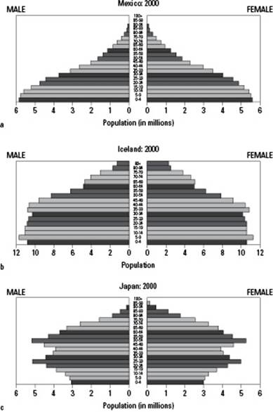
Figure 11-3: A survivorship curve.
Discovering how populations grow
Populations have the potential to grow exponentially when organisms have more than one offspring. Why? Because those offspring have offspring, and the population gets even bigger.
For example, assume 1 organism has 3 offspring, creating a population of 4 organisms. Say each of the 3 original offspring has 3 offspring, adding 9 and bringing the total population to 13 organisms. If the 9 newest offspring have 3 offspring each, that adds 27 new individuals and brings the total population to 40. Although the rate of reproduction per individual, called the per capita reproduction rate, remains the same, the population grows larger and larger.
The next sections fill you in on the factors that affect population growth, how scientists track a population’s growth, and more.
Understanding biotic potential
The maximum growth rate of a population under ideal conditions is referred to as biotic potential. Ideal conditions occur when species don’t have to compete for resources, such as food or water, and when no predators or diseases affect the growth of the organisms. Other factors involved in determining biotic potential include
The age of the organisms when they’re able to reproduce
The number of offspring typically produced from one successful mating
How often the organisms reproduce
How long a period of time they’re capable of reproducing
The number of offspring that survive to adulthood
Bacteria, for example, have a very high biotic potential. Many bacteria can reproduce in less than an hour, and their offspring are ready to begin reproduction as soon as they’re made. If one cell of E. coli could grow without limits for just 48 hours, the population of bacteria produced would weigh the same amount as the Earth!
Looking at the factors affecting population growth
Population growth can be limited by a number of environmental factors, which population ecologists group into two categories:
Density-dependent factors are more likely to limit growth as population density increases. For example, large populations may not have enough food, water, or nest sites, causing fewer organisms to survive and reproduce. This lower birth rate combines with a higher death rate to slow population growth.
Density-independent factors limit growth but aren’t affected by population density. Changes in weather patterns that cause droughts or natural disasters such as earthquakes kill individuals in populations regardless of that population’s size.
Some populations can remain very steady in the face of these factors, whereas others fluctuate quite a bit.
Populations that depend on limited resources fluctuate more than populations that have ample resources. If a population depends heavily on one type of food, for example, and that food becomes unavailable, the death rate will increase rapidly.
Populations with low reproductive rates are more stable than populations with high reproductive rates. Organisms with high reproductive rates may have sudden booms in population as conditions change. Organisms with low reproductive rates don’t experience these booms; their population growth rate is fairly steady.
Populations may rise and fall because of interactions between predators and prey. When prey is abundant, predator populations grow until the increased numbers of predators eat up all the prey. When that happens, the prey population crashes, followed by the predator population as the predators starve. After the predator population crashes, the prey has a chance to recover, and its numbers increase again, starting the cycle anew.
Reaching carrying capacity
When a population hits carrying capacity, it has reached the maximum amount of organisms of a single population that can survive in one habitat (the scientific name for a home).
As populations approach the carrying capacity of a particular environment, density-dependent factors have a greater effect, and population growth slows dramatically. If carrying capacity is exceeded even temporarily, the habitat may be damaged, further reducing the amount of resources available and leading to increased deaths. This situation decreases the population so that the carrying capacity can be met once again. However, if the habitat is damaged, the carrying capacity may be lowered even further, necessitating even more deaths to restore balance.
Graphing growth rates
Scientists often use graphs to make sense of population data. J-shaped growth curves, like the one in Figure 11-4a, depict exponential growth. In other words, they show that a population is increasing at a steady rate (the birth and death rates are constant). In nature, populations may show exponential growth for short periods of time, but then environmental factors act to limit their growth rate.
S-shaped growth curves, like the one in Figure 11-4b, show logistic growth, meaning the population size is affected by environmental factors. In logistic growth, the growth rate is high when population density is low and then slows as population density increases.
Painting with numbers: Using statistics to get a picture of population growth
Population ecologists use statistics to model the growth of populations. The natural growth rate of a population (r) is equal to the per capita birth rate (b) minus the per capita death rate (d). In other words: r = b – d.
If migration is occurring, meaning organisms are moving from one place to another, immigration is added to the birth rate, and emigration is added to the death rate. When conditions are optimal, the growth rate reaches its maximum and is called the intrinsic rate of increase, or rmax. Different species have characteristic values for rmax. For example, even if conditions are optimal, the rmax of elephants is never going to be close to the rmax for E. coli.
The growth rate of any population at a particular time can be calculated by multiplying the intrinsic rate of increase (rmax) by the number of individuals in the population (N). In other words: ΔN÷Δt = Nrmax.
Figure 11-4:Population growth curves.

Taking a closer look at the human population
There’s no doubt about it: Humans are the dominant population on Earth, and our numbers keep on rising. It’s important to have an understanding of how our population is growing because of the impact humans have on the planet and all the other species on it. The following sections provide some insight into this and introduce you to the special tool population ecologists have derived to study human population growth.
The human population explosion
Up until about a thousand years ago, human population growth was very stable. Food wasn’t as readily available as it is now. Nor were there antibiotics to fend off invading bacteria, vaccines to fight against deadly diseases, and sewage treatment plants to ensure that water was safe to drink. People didn’t shower or wash their hands as often, so they spread diseases more easily. All of these factors, and more, increased the death rate and decreased the birth rate of the human population.
Yet in the last 100 to 200 years, the food supply has increased and hygiene and medicines have reduced deaths due to common illnesses and diseases. So not only are more people born, but more of these people are surviving well past middle age. As you can see in Figure 11-5, the human population has grown exponentially in relatively recent history.
Figure 11-5:Human population growth.
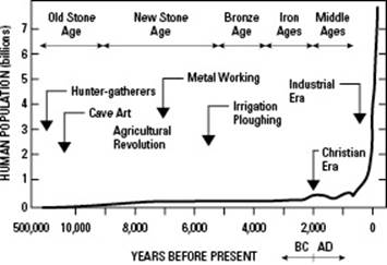
If Figure 11-5 doesn’t impress you, here are a few statistics that might:
The human population doubled in the 40 years between 1950 and 1990.
Every second, about three new people are born.
The global human population passed the 6 billion mark at the end of the 20th century.
At current growth rates, the human population is projected to reach 8 to 12 billion by the end of the 21st century. Imagine that for a minute. What would your life be like if twice as many people lived on Earth as do today? There’d be twice as many people dining at restaurants, driving around, going to the movies, hiking in the woods . . . you get the idea.
What’s scary is that scientists question whether the Earth can even support that many humans. The exact carrying capacity of the Earth for humans isn’t known because, unlike other species, humans can use technology to increase the Earth’s carrying capacity for the species. Currently, scientists estimate that humans are using about 19 percent of the Earth’s primary productivity, which is the ability of living things like plants to make food. Humans also use about half of the world’s freshwater. If humans continue to use more and more of the Earth’s resources, the increased competition will drive many other species to extinction. (This pressure on other species from human impacts is already being seen, endangering species such as gorillas, cheetahs, lions, tigers, sharks, and killer whales.)
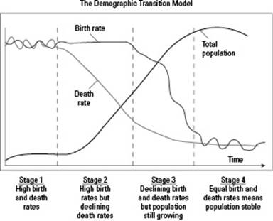
The demographic transition model
Comprehending human population growth is a bit tougher than following the population growth of other organisms. Technology, education, and other factors affect how different human populations grow. Richer, industrialized nations (such as European countries, the United States, and Iceland), have reached a stage of zero population growth, meaning birth and death rates are equal in these countries. On the other hand, poorer, less industrialized nations (such as many countries in Africa) have very high birth rates relative to their death rates and have rapidly growing populations.
The major difference between these groups of nations is fertility. In less industrialized nations, families that have more children gain an economic benefit because the children are needed for labor-intensive tasks. In more industrialized nations, fewer children are needed to work for the family, and raising children becomes more expensive, so people choose to have fewer children.
Population ecologists have developed a special demographic transition model to note the stages of development the human population goes through in any given country on its way to stabilization. Based on human history over the past century or so, the process to reach full demographic transition has four stages (see Figure 11-6 for the visual):
Stage 1: Birth and death rates are both high. Basic sanitation and modern medicine aren’t yet available to lower the death rate and extend the life span. Demographic transition has not yet occurred.
Stage 2: Sanitation and medicine lower the death rate, but the economy still encourages a high birth rate. Farming remains a large part of the economy in Mexico, for example, so many people there still have large families.
Stage 3: Increased urbanization reduces the need for large families, and the cost of raising and educating children encourages fewer births. The birth rate drops and becomes close to that of the death rate. The population still grows, however, as earlier generations reach reproductive age. As countries pass from Stage 2 to Stage 3, they make a partial demographic transition.
Stage 4: The population becomes stable, and birth rates equal death rates. When countries reach Stage 4, they’ve made a full demographic transition.
Figure 11-6: The demographic transition model.
Moving Energy and Matter around within Ecosystems
Organisms interact with their environment and with other organisms to acquire energy and matter for growth. The interactions between organisms influence behavior and help the organisms establish complex relationships.
One of the most fundamental ways that organisms interact with each other is eating each other. In fact, all the various organisms in an ecosystem can be divided into four categories called trophic levels based on how they get their food:
Producers make their own food. Plants, algae, and green bacteria are all producers that use energy from the Sun to combine carbon dioxide and water and form carbohydrates via photosynthesis. Producers can also be called autotrophs (see Chapter 5 for more on autotrophs and the process of photosynthesis).
Primary consumers eat producers. Because producers are mainly plants, primary consumers are also called herbivores (plant-eating animals).
Secondary consumers eat primary consumers. Because primary consumers are animals, secondary consumers are also called carnivores (meat-eating animals).
Tertiary consumers eat secondary consumers, so they’re also considered carnivores.
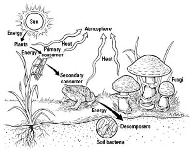
Organisms in the different trophic levels are linked together in a food chain, a sequence of organisms in a community in which each organism feeds on the one below it in the chain. Figure 11-7 shows a depiction of a simple food chain.
Figure 11-7:Energy flow in ecosystems shown through a food chain.
Interactions in ecosystems go way beyond those shown in a simple food chain because
Some organisms eat at more than one trophic level. You, for example, may eat a slice of pizza with pepperoni. The grain that made the crust came from a plant, so when you eat the crust you’re acting as a primary consumer. The pepperoni, however, came from an animal, so when you eat the pepperoni, you’re acting as a secondary consumer.
Some organisms eat more than one type of food. When you eat pepperoni pizza, you’re eating food from both plants and animals. Organisms such as humans that eat both plants and animals are called omnivores. Also, organisms that eat more than one type of food belong to more than one food chain. When all the food chains from an ecosystem are put together, they form an interconnected food web.
Some organisms get their food by breaking down dead things. Decomposers, like bacteria and fungi, release enzymes onto dead organisms, breaking them down into smaller components for absorption. Detritivores, such as worms, small insects, crabs, and vultures, also eat the dead.
The sections that follow delve into the details of how energy and matter move from one organism to another in a never-ending cycle that’s essential to the survival of life on this planet.
Going with the (energy) flow
The energy living things need to grow flows from one organism to another through food. Sounds simple, we know, but that energy is governed by a few key principles, perhaps most important of which is that an organism never gets to use the full amount of energy it receives from the thing it’s “eating.”
In the sections that follow, we reveal the principles that govern energy as well as the way in which scientists measure the flow of energy from organisms at different levels of the food chain.
Energy principles
Some really important energy principles form the foundation of organism interactions in ecosystems:
Energy can’t be created or destroyed. This statement represents a fundamental law of the universe called the First Law of Thermodynamics. The consequence of this law is that every living thing has to get its energy from somewhere. No living thing can make the energy it needs all by itself. Even producers, who make their own food, can’t make their own energy — they capture energy from the environment and store it in the food they make.
When energy is moved from one place to another, it’s transferred. When a primary consumer eats a producer, the energy that was stored in the body of the producer is transferred to the primary consumer.
When describing energy transfers, be sure to say where the energy is coming from and where it’s going to.
When energy is changed from one form to another, it’s transformed. When plants do photosynthesis, they absorb light energy from the Sun and convert it into the chemical energy stored in carbohydrates. So, during photosynthesis, light energy is transformed into chemical energy.
When describing energy transformations, be sure to state the form of energy both before and after the transformation.
When energy is transferred in living systems, some of the energy is transformed into heat energy. This statement is one way of representing another law of the universe, called the Second Law of Thermodynamics. The impact of this law on ecosystems is that no energy transfer is 100 percent efficient. After energy is transferred to heat, it’s no longer useful as a source of energy to living things. In fact, only about 10 percent of the energy available at one trophic level is usable to the next trophic level.
The Second Law of Thermodynamics has many impacts on energy and can be stated in several different ways. In biology, it’s usually stated as “all chemical reactions spontaneously occur in the direction that increases disorder (called entropy) in the universe.” What this means is that any process that makes things more random — like breaking down molecules or spreading molecules randomly over an area — can occur without the input of energy. This tendency of the universe to become more random also applies to the distribution of energy. Food molecules represent a very concentrated form of energy — that’s why living things like them so much. Heat, on the other hand, is a much more dispersed, or random, form of energy. So, according to the Second Law of Thermodynamics, if energy from food molecules is involved in an energy transfer, some of that energy is going to become more randomly dispersed, meaning it transforms into heat energy.
You may hear people, even scientists, say that “energy is lost” or “energy is lost as heat.” These statements can be confusing because they make it sound like energy disappears somehow. But you know from the First Law of Thermodynamics that energy can’t be destroyed or disappear. The correct interpretation of statements like these is that useful energy is lost from the system as it’s transformed into heat. In other words, after energy is transformed into heat, organisms in an ecosystem can’t use it as a source of energy for growth.
 Never use the words lost, disappear, destroyed, or created when you’re talking about energy. Use the words transfer and transformed instead, and you’ll avoid a great deal of confusion.
The energy pyramid
Scientists use an energy pyramid (also called a trophic pyramid; see Figure 11-8) to illustrate the flow of energy from one trophic level to the next. Energy pyramids show the amount of energy at each trophic level in proportion to the next trophic level — what ecologists refer to asecological efficiency. To estimate ecological efficiency, ecologists use a rule of thumb called the 10-percent rule, which says that only about 10 percent of the energy available to one trophic level gets transferred to the next trophic level.
Figure 11-8: The energy pyramid.
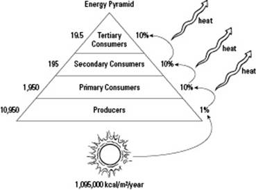
Following along in Figure 11-8, you see that energy travels to the Earth from the Sun. About 1 percent of the energy available to producers is captured and stored in food. Producers grow, transferring much of their stored energy into ATP for cellular work (as explained in Chapter 5) and the molecules that make up their bodies. As producers transfer energy for growth, some energy is also transformed into heat that’s transferred to the environment.
About 10 percent of the energy that was originally stored in producers is transferred to primary consumers when they eat the producers. Just like producers, the primary consumers grow, transferring energy from food into ATP for cellular work and into the molecules that make up their bodies. As primary consumers transfer energy for growth, some energy is also transformed into heat that’s transferred to the environment. This process repeats itself when secondary consumers eat primary consumers and when tertiary consumers eat secondary consumers. Each level of consumer receives about 10 percent of the energy originally captured by the organism it consumed, and as the consumer uses energy for growth, it transfers some of that energy back to the environment as heat.
But the energy pyramid doesn’t end there. As organisms die, some of their remains become part of the environment. Decomposers and detritivores use this dead matter as their source of food, transferring energy from food into ATP and molecules and giving off some energy as heat.
Note: Food chains and energy pyramids usually don’t go beyond tertiary consumers because the amount of energy available to each level is reduced as you move up the pyramid. Past the tertiary consumer level, too much energy has been depleted from the system.
Cycling matter through ecosystems
Not only does food provide energy to living things (as explained earlier in this chapter) but it also provides the matter organisms need to grow, repair themselves, and reproduce. For example, you eat food that contains proteins, carbohydrates, and fats, and your body is made of proteins, carbohydrates, and fats (see Chapter 3 for more on these molecules). When you eat food, you break it down through digestion (covered in Chapter 16) and then transfer small food molecules around your body via circulation (covered in Chapter 15) so that all of your cells receive food. Your cells then have two options:
They can use the food for energy by breaking it down into carbon dioxide and water through cellular respiration (see Chapter 5).
They can rebuild the small food molecules into the larger food molecules that make up your body.
Yes, that second option means you are what you eat — well, almost. You don’t use food molecules directly to build your cells; you break them down first and use the pieces to build what you need. In other words, your cells are made of human molecules that are rebuilt from the parts of molecules taken from the plants and animals you’ve eaten. So really you’re made of molecules that you recycled from your food. (Likewise, the living things your food used to be got their molecules by recycling them from somewhere else.)
Think about what all goes into a slice of pepperoni pizza. The crust came from the grains of plants, and the pepperoni (for the sake of argument) came from a pig. Plants make their own food from carbon dioxide and water and then use that food to build their bodies, which means the plant that went into your pizza crust got the parts it needed to build its body from carbon dioxide in the air and water in the soil. Pigs get their molecules by eating whatever food the farmer gives them, which is likely some type of plant. After you eat a slice of pepperoni pizza, you can trace some of the atoms that make up your body back to carbon dioxide from the air, water from the soil, and plants that were fed to pigs.
One of the most fascinating facts about the Earth is that almost all the matter on this planet today has been here since the Earth first formed. That means all the carbon, hydrogen, oxygen, nitrogen, and other elements that make up the molecules of living things have been recycled over and over throughout time. Consequently, ecologists say that matter cycles through ecosystems.
Scientists track the recycling of atoms through cycles called biogeochemical cycles (bio because the recycling involves living things, geo because it involves the Earth, and chemical because it involves chemical processes). Four biogeochemical cycles that are particularly important to living things are the hydrologic cycle, the carbon cycle, the phosphorous cycle, and the nitrogen cycle.
The hydrologic cycle
The hydrologic cycle (also known as the water cycle) refers to plants obtaining water by absorbing it from the soil and animals obtaining water by drinking it or eating other animals that are made mostly of water. Water returns to the environment when plants transpire (as explained in Chapter 21) and animals perspire. Water evaporates into the air and is carried around the Earth by wind. As moist air rises and cools, water condenses again and returns to the Earth’s surface as precipitation (think rain, snow, sleet, and hail). Water moves over the Earth’s surface in bodies of water such as lakes, rivers, oceans, and even glaciers; it also moves through the groundwater below the soil.
The carbon cycle
The carbon cycle (depicted in Figure 11-9) may be the most important biogeochemical cycle to living things because the proteins, carbohydrates, and fats that make up their bodies all have a carbon backbone (see Chapter 3 for more on these molecules). In the carbon cycle, plants take in carbon dioxide from the atmosphere, using it to build carbohydrates via photosynthesis (covered in Chapter 5). Animals consume plants or other animals, incorporating the carbon that was in their food molecules into the molecules that make up their own bodies. Decomposers break down dead material, incorporating the carbon from the dead matter into their bodies.
Figure 11-9: The carbon cycle.
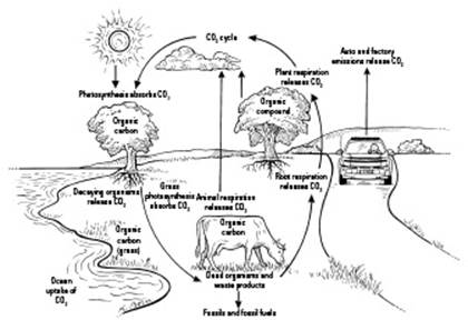
All of these living things — producers, consumers, and decomposers — also use food molecules as a source of energy, breaking the food molecules back down into carbon dioxide and water in the process of cellular respiration (see Chapter 5). Cellular respiration releases the carbon atoms back into the environment as carbon dioxide, where it’s again available to producers for photosynthesis.
Carbon storage in living things (in the form of proteins, carbohydrates, and fats) is purely temporary. Carbon can actually be stored in the environment for longer periods of time.
Large forests represent significant storage of carbon, which can be suddenly released back to the environment as carbon dioxide when forests are cut and wood is burned.
Fossil fuels contain carbon that was stored in the bodies of living things long ago and then trapped in a way that the proteins, carbohydrates, and fats were converted to coal, oil, and natural gas deposits. As people burn fossil fuels, this stored carbon is being rapidly released back into the atmosphere as carbon dioxide, causing the concentration of carbon dioxide in the atmosphere to rise to its highest levels in recorded history.
Carbon is also stored in the world’s oceans, in the form of dissolved carbon dioxide. Warm water holds less carbon dioxide than cold water, so some of this carbon may be released back to the atmosphere if ocean temperatures rise as a result of global warming.
The phosphorus cycle
Phosphorous is an important component of the molecules that make up living things. It’s found in adenosine triphosphate (ATP), the energy-storing molecule produced by every living thing, as well as the backbones of DNA and RNA molecules. The phosphorous cycle involves plants obtaining phosphorous when they absorb inorganic phosphate and water from the soil and animals obtaining phosphorous when they eat plants or other animals. Phosphorus is excreted through the waste products created by animals, and it’s released by decomposers back into the soil as they break down dead materials. When phosphorus gets returned to the soil, it’s either absorbed again by plants or it becomes part of the sediment layers that eventually form rocks. As rocks erode by the action of water, phosphorus is returned to water and soil.
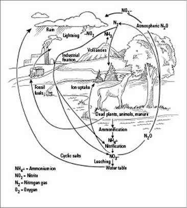
The nitrogen cycle
Not only is nitrogen part of the amino acids that make up proteins but it’s also found in DNA and RNA (see Chapter 3 for more on these molecules). Nitrogen also exists in several inorganic forms in the environment, such as nitrogen gas (in the atmosphere) and ammonia or nitrates (in the soil).
Because nitrogen exists in so many forms, the nitrogen cycle (shown in Figure 11-10) is pretty complex.
Nitrogen fixation occurs when atmospheric nitrogen is changed into a form that’s usable by living things. Nitrogen gas in the atmosphere can’t be incorporated into the molecules of living things, so all the organisms on Earth depend upon the activity of bacteria that live in the soil and in the roots of plants. These nitrogen-fixing bacteria convert nitrogen gas (N2) into forms such as ammonium ion or nitrate (NH4+ or NO3–) that organisms can use. Plants obtain nitrogen by absorbing ammonia and nitrate along with water from the soil; animals get their nitrogen by eating plants or other animals.
Some nitrogen fixation also occurs via lightning strikes and processes in factories that produce chemical fertilizers for plants. However, the nitrogen fixation that occurs from lightning strikes isn’t enough to supply ecosystems with all the nitrogen they need, and industrial nitrogen fixation requires a lot of energy.
Ammonification releases ammonia into the soil. As decomposers break down the proteins in dead things, they may not need all the nitrogen from those proteins for themselves. If the decomposers have excess nitrogen, they release some of it into the soil as ammonia (NH3). In the soil, ammonia converts into ammonium ion (NH4+). The waste products of animals also contain nitrogen in the form of urea or uric acid that can be converted to ammonia by bacteria living in the soil.
Nitrification converts ammonia to nitrite and nitrate. Certain bacteria get their energy by converting ammonia (NH3) into nitrite (NO2–). Other bacteria get their energy by converting the NO2– into nitrate (NO3–).
Denitrification converts nitrate to nitrite and nitrogen gas. Some bacteria in the soil use nitrate (NO3–) rather than oxygen for cellular respiration (see Chapter 5 for more on cellular respiration). When these bacteria use nitrate, they convert it into nitrite that’s released into the soil or nitrogen gas that’s released into the atmosphere.
Figure 11-10:The nitrogen cycle.