MCAT Biology Review

Chapter 12: Genetics and Evolution

12.3 Analytical Approaches in Genetics

Genetics is a field in which a number of analytical approaches, mostly focused on statistical analysis, have been developed. These range from the Punnett square to mapping of chromosomes with recombinant frequencies to Hardy–Weinberg equilibrium.

PUNNETT SQUARES

Punnett squares are diagrams that predict the relative genotypic and phenotypic frequencies that will result from the crossing of two individuals. The alleles of the two parents are arranged on the top and side of the square, with the genotypes of the progeny represented at the intersections of these alleles. The genotypes of the progeny will be the sum of the two parental alleles.

MCAT EXPERTISE

Pedigree (or family tree) analysis was once a mainstay of MCAT passages and questions. While this topic no longer appears on the exam, it will be a major focus of your medical school genetics class. The symbology of pedigree analysis is complex and intricate, but a great deal of information can be gleaned from a well-drawn pedigree.

Monohybrid Cross

In genetics problems, including those on the MCAT, dominant alleles are assigned capital letters and recessive alleles are assigned lowercase letters. If both copies of the allele are the same, that individual is said to be homozygous. If they are different, the individual is heterozygous.

A cross in which only one trait is being studied is said to be monohybrid. The parent or P generation refers to the individuals being crossed; the offspring are the filial or F generation. Multiple generations can be denoted F generations by using numeric subscripts. If you think of your grandparents as the P generation, then your parents are in the F₁ generation, and you are in the F₂ generation.

Mendel worked with pea plants that had either purple or white flowers. Before crossing the different plants, each group contained homozygotes; subsequent experimentation revealed that the allele for purple color was dominant (P) and the allele for white color was recessive (p). Thus, crossing a purple flower with a white flower would be crossing PP with pp, resulting in an F₁ generation that contained 100 percent Pp or heterozygotes, as shown in Figure 12.5. All of the flowers in this generation would be purple because P is a dominant allele.

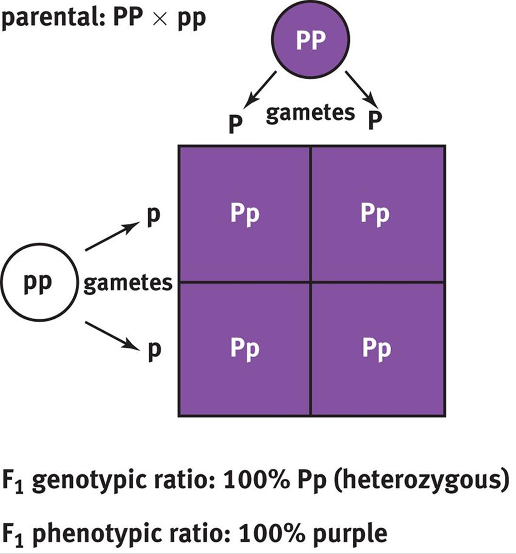Figure 12.5. Punnett Square of Homozygous Parents

If two members of the F₁ generation were crossed, the resulting offspring in the F₂ generation would be more genotypically and phenotypically diverse than their parents. Crossing two plants with the genotype Pp would result in 25 percent PP, 50 percent Pp, and 25 percent pp offspring, as shown in Figure 12.6. Phenotypically, this would be a 3:1 distribution because both the homozygous dominant and heterozygous dominant offspring would be purple-flowering plants. Thus, crossing two heterozygotes in a case of complete dominance will result in a 1:2:1 distribution of genotypes (homozygous dominant:heterozygous dominant:homozygous recessive) and a 3:1 distribution of phenotypes (dominant:recessive). These ratios are, of course, theoretical probabilities and will not always hold true—especially in a small population of offspring. Usually, the more offspring that parents have, the closer their phenotypic ratios will be to the expected ratios.

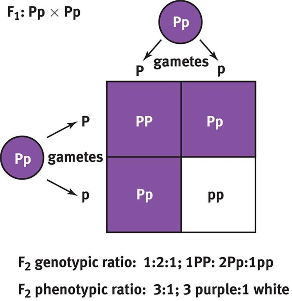Figure 12.6. Punnett Square of Heterozygous Parents

KEY CONCEPT

Crossing two heterozygotes for a trait with complete dominance results in a 1:2:1 ratio of genotypes and a 3:1 ratio of phenotypes. Know these ratios cold for Test Day!

MCAT EXPERTISE

The ability to create and read a Punnett square quickly on Test Day is one of the most useful skills for questions involving Mendelian inheritance. Often, an entire passage in the Biological and Biochemical Foundations of Living Systems section will be devoted to classical and molecular genetics and will require the use of at least one Punnett square.

Test Cross

A test cross is used to determine an unknown genotype, as shown in Figure 12.7. In a test cross, the organism with an unknown genotype is crossed with an organism known to be homozygous recessive. If all of the offspring (100 percent) are of the dominant phenotype, then the unknown genotype is likely to be homozygous dominant. If there is a 1:1 distribution of dominant to recessive phenotypes, then the unknown genotype is likely to be heterozygous. Because a test cross is used to determine the genotype of the parent based on the phenotypes of its offspring, test crosses are sometimes called back crosses.

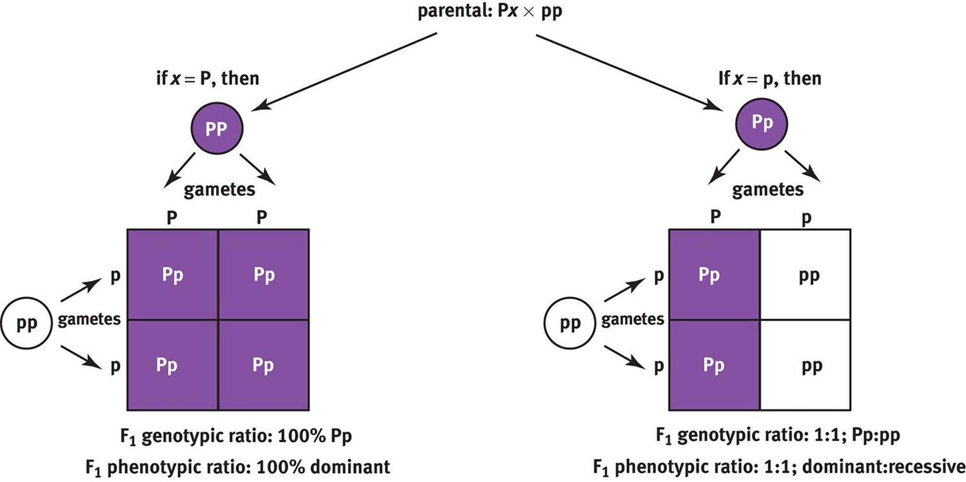Figure 12.7. Test Cross An organism with an unknown genotype is crossed with a homozygous recessive organism to identify the unknown genotype using the resulting offspring.

Dihybrid Cross

We can extend a Punnett square to account for the inheritance of two different genes using a dihybrid cross. Remember that, according to Mendel’s second law (of independent assortment), the inheritance of one gene is independent of the inheritance of the other. This will hold true forunlinked genes, although it will be more complicated for linked genes, as described later in this chapter.

If we expand the previous crosses to consider not only flower color, but also plant height, then we can create a 4 × 4 Punnett square, as shown in Figure 12.8. Remember that purple is dominant (P) and white is recessive (p); similarly, tall is dominant (T) and short or dwarf is recessive (t). If we cross two plants that are heterozygous for both traits, then the offspring have a phenotypic ratio of 9:3:3:1 (9 tall and purple:3 tall and white:3 dwarf and purple:1 dwarf and white). Note that the 3:1 phenotypic ratio still holds for each trait (12 tall:4 dwarf and 12 purple:4 white), reflecting Mendel’s second law.

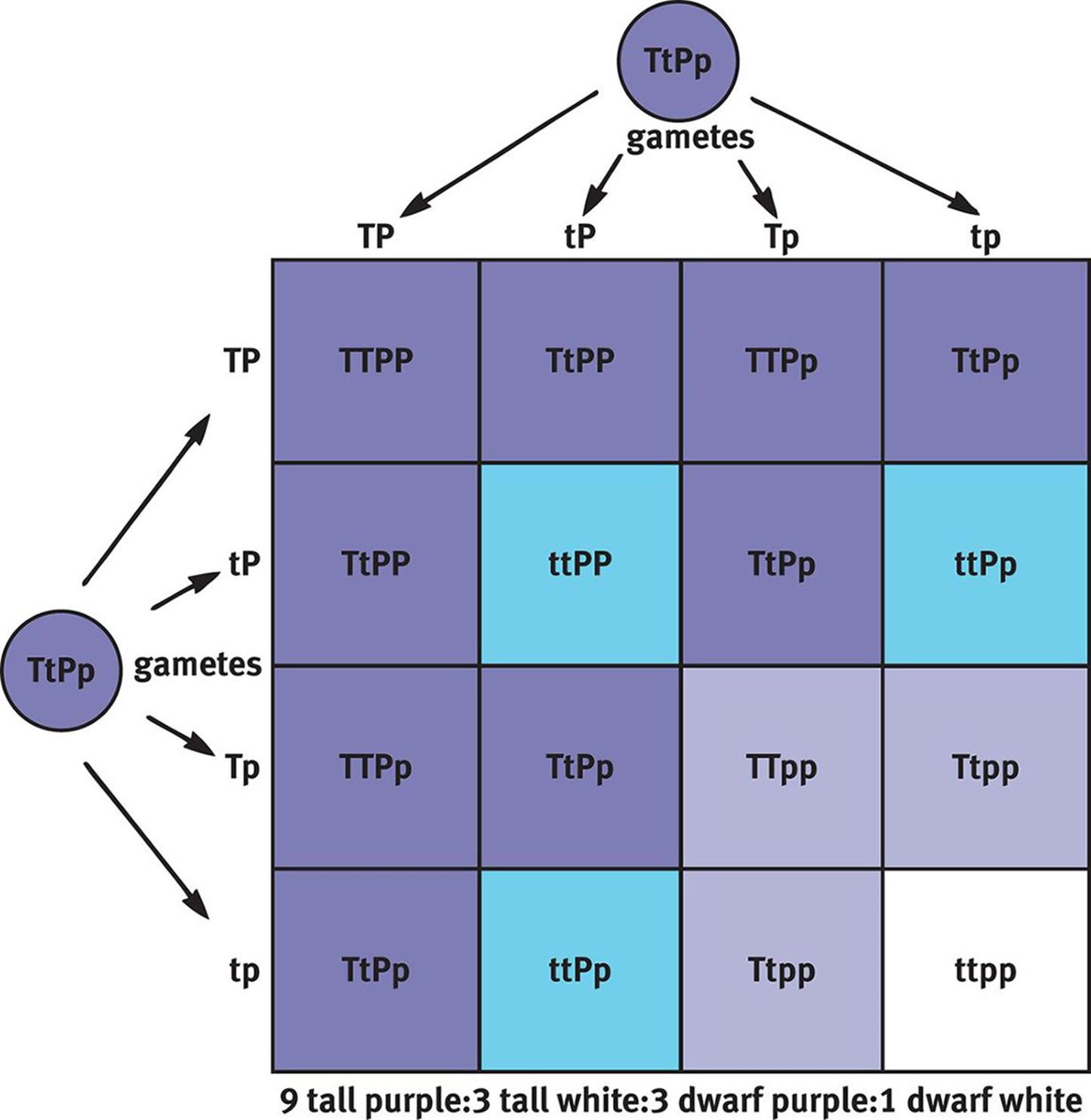Figure 12.8. Dihybrid Cross

MCAT EXPERTISE

Just as with the 3:1 phenotypic ratio of a monohybrid cross, it is worth memorizing the 9:3:3:1 distribution for dihybrid crosses between two heterozygotes with complete dominance.

Sex-Linked Crosses

When considering sex-linked (X-linked) traits, a slightly different system is used to symbolize the various alleles. This is because females have two X chromosomes and thus may be homozygous or heterozygous for a condition carried on the X chromosome. Males, on the other hand, have only one X chromosome (and one Y chromosome) and are hemizygous for many genes carried on the X chromosome. This is why sex-linked traits are much more common in males; having only one recessive allele is sufficient for expression of the recessive phenotype.

MNEMONIC

On the MCAT, sex-linked is X-linked. Y-linked diseases exist, but are exceedingly rare. Further, unless told otherwise, assume that sex-linked traits are recessive.

When writing genotypes for sex-linked traits, we use X and Y to symbolize normal X and Y chromosomes. An X chromosome carrying an affected allele is commonly given a subscript, such as X_a, to indicate the presence of the disease-carrying allele. Hemophilia is a particularly common example of a sex-linked trait; a Punnett square for a heterozygous (carrier) female and both a normal male and affected (hemophiliac) male are shown in Figure 12.9.

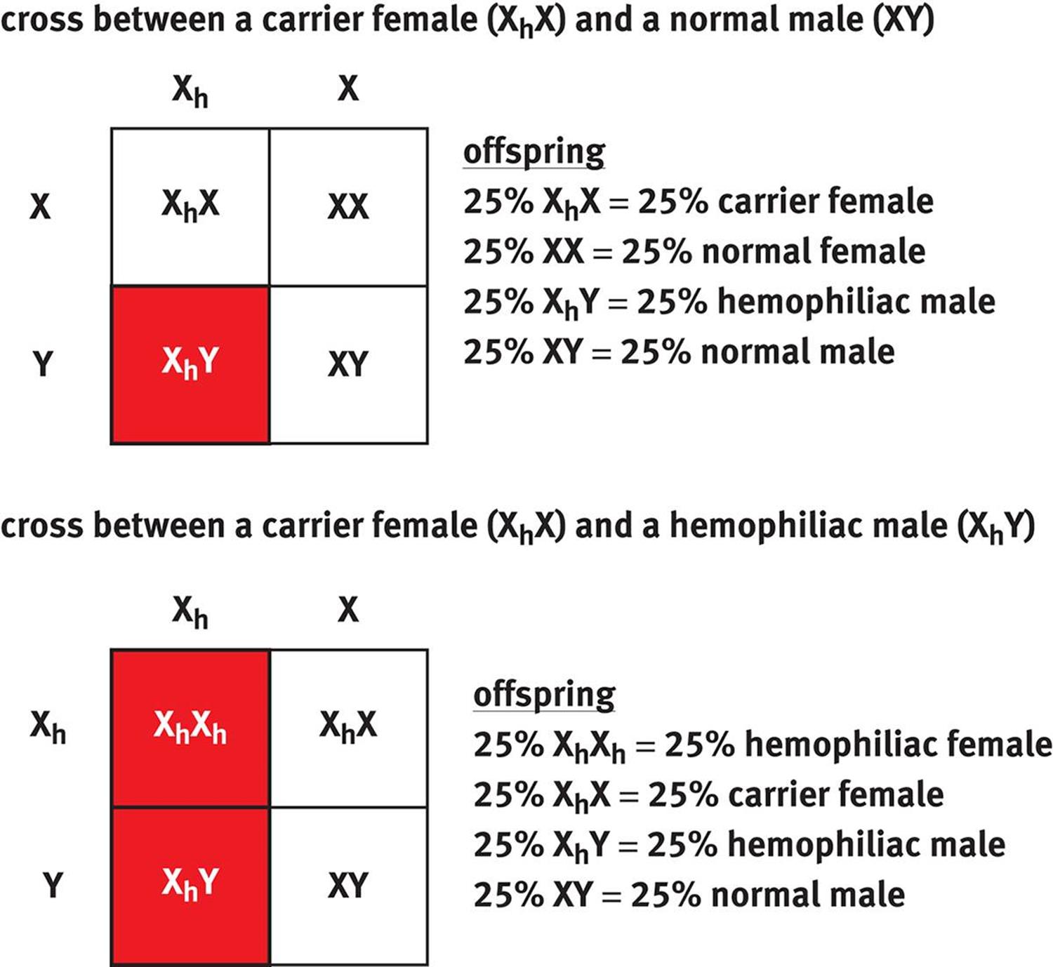Figure 12.9. Sex-Linked Cross Unless stated otherwise, assume that all sex-linked traits on the MCAT are X-linked recessive.

KEY CONCEPT

Because an egg necessarily carries an X chromosome, it is the sperm that determines the sex of a child. It follows that men with a sex-linked trait will have daughters who are all either carriers of the trait or who express the trait (if his partner also has an affected allele), and that a man can never pass down a sex-linked trait to his son.

GENE MAPPING

Genes are organized in a linear fashion on chromosomes. As discussed earlier, crossing over during prophase I of meiosis causes alleles to be swapped between homologous chromosomes, supporting Mendel’s second law (of independent assortment). However, genes that are located very close together on a chromosome are less likely to be separated from each other during crossing over. In other words, the further apart two genes are, the more likely it is that there will be a point of crossing over, called a chiasma, between them. The likelihood that two alleles are separated from each other during crossing over, called the recombination frequency (θ), is roughly proportional to the distance between the genes on the chromosome. We can also describe the strength of linkage between genes based on the recombination frequency: tightly linked genes have recombination frequencies close to 0 percent; weakly linked genes have recombination frequencies approaching 50 percent, as expected from independent assortment.

By analyzing recombination frequencies, a genetic map that represents the relative distance between genes on a chromosome can be constructed. By convention, one map unit or centimorgan corresponds to a 1 percent chance of recombination occurring between two genes. Thus, if two genes were 25 map units apart, we would expect 25 percent of the total gametes examined to show recombination somewhere between these two genes. Recombination frequencies can be added in a crude approximation to determine the order of genes in the chromosome, as shown in Figure 12.10.

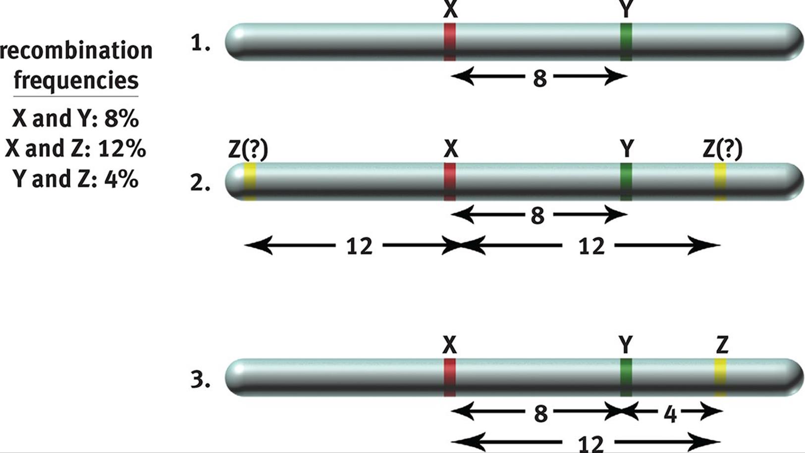Figure 12.10. Genetic Maps from Recombination Frequencies If the recombination frequencies are known, one can deduce the order of genes on the chromosome because map units are roughly additive.

HARDY–WEINBERG PRINCIPLE

How often an allele appears in a population is known as its allele frequency. For example, if we took a one-cell sample from 50 of Mendel’s plants, we could collect 100 copies of alleles for flower color (two from each cell). If 75 of these alleles were the dominant allele, we could say that the allele frequency of P is 75 ÷ 100 = 0.75. Note that this does not indicate which flowers contain the allele, or if those flowers are homozygous or heterozygous; it only tells us the representation of the allele across all chromosomes in the population. Evolution results from changes in these gene frequencies in reproducing populations over time. However, when the gene frequencies of a population are not changing, the gene pool is stable, and evolution is ostensibly not occurring. Five criteria must be met for this to be possible:

· The population is very large (no genetic drift).

· There are no mutations that affect the gene pool.

· Mating between individuals in the population is random (no sexual selection).

· There is no migration of individuals into or out of the population.

· The genes in the population are all equally successful at reproducing.

Provided that all of these conditions are met, the population is said to be in Hardy–Weinberg equilibrium, and a pair of equations can be used to predict the allelic and phenotypic frequencies.

Let us define a particular gene as having only two possible alleles, T and t. We will define p to be the frequency of the dominant allele T and q to be the frequency of the recessive allele t. Because there are only these two choices at the same gene locus, p + q = 1. That is, the combined allele frequencies of T and t must equal 100 percent. If we square both sides of the equation, we get:

(p + q)² = 1²
p² + 2pq + q² = 1

where p² is the frequency of the TT (homozygous dominant) genotype, 2pq is the frequency of the Tt (heterozygous dominant) genotype, and q² is the frequency of the tt (homozygous recessive) genotype. Note that the sum p² + 2pq would represent the frequency of the dominant phenotype(both homozygous and heterozygous dominant genotypes).

KEY CONCEPT

All you need to know to solve any MCAT Hardy–Weinberg problem is the value of p (or p²) or q (or q²). From there, you can calculate everything else using p + q = 1 and p² + 2pq + q² = 1.

For Test Day, you should be aware of the two key Hardy–Weinberg equations demonstrated above:

p + q = 1
p² + 2pq + q² = 1

Equation 12.1

We should be aware that each equation provides us with different information. The first tells us about the frequency of alleles in the population, whereas the second provides information about the frequency of genotypes and phenotypes in the population.

KEY CONCEPT

Hardy–Weinberg equations allow you to find two pieces of information: first, the relative frequency of alleles in a population and, second, the frequency of a given genotype or phenotype in the population. Remember that there will be twice as many alleles as individuals in a population—because each individual has two autosomal copies of each gene.

These equations can also be used to demonstrate that evolution is not occurring in a population. Assuming that the conditions listed earlier are met, the allele frequencies will remain constant from generation to generation. For example, imagine that we have a population of Mendel’s pea plants in which the frequency of the tall allele, T, is 0.80. This value is represented by p. This means that q (the short allele, t) is 0.20 by subtraction. Setting up our F₁ cross for two heterozygotes, we can see the results of such a mating:

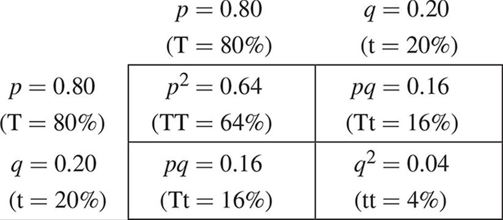
We see that the filial generation contains 64 percent homozygous tall, 32 percent heterozygous tall, and 4 percent homozygous short plants. These are the genotypic frequencies. We can determine the allele frequencies in this generation as follows:

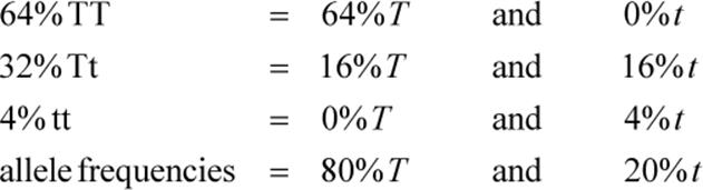
Notice that the allele frequencies are unchanged compared to the parent generation. T is still 0.80 and t is still 0.20. Populations in Hardy–Weinberg equilibrium will exhibit this property.

MCAT Concept Check 12.3:

Before you move on, assess your understanding of the material with these questions.

1. For each of the crosses below, what is the phenotypic ratio seen in the offspring?

2. If genes Q and R have a recombination frequency of 2%, genes R and S have a recombination frequency of 6%, genes S and T have a recombination frequency of 23%, and genes Q and T have a recombination frequency of 19%, then what is the order of these four genes in the chromosome?

3. All five criteria of the Hardy–Weinberg principle are required to imply what characteristic of the study population?

4. Assume that a population is in Hardy–Weinberg equilibrium. If 9% of the population is homozygous dominant, then solve for the following:

· The frequency of the dominant allele:

· The frequency of the recessive allele:

· The fraction of the population that is heterozygous:

· The fraction of the population with a homozygous recessive genotype:

· The fraction of the population with a dominant phenotype: