CHEMICAL BIOLOGY
Förster Resonance Energy Transfer (FRET) for Proteins
Lambert K. Chao and Robert M. Clegg, Physics Department,
University of Illinois-Urbana-Champaign, Urbana, Illinois
doi: 10.1002/9780470048672.wecb171
Förster Resonance Energy Transfer (FRET) is a spectroscopic technique applied throughout physics, chemistry, and biology to measure quantitatively the distance between selected locations on macromolecules and to determine the close association between interacting molecular components. Because FRET typically occurs over distances from 0.5 to 10 nm, it is especially useful for investigating many interesting biological molecular structures. It is also particularly valuable for following the dynamics and structural fluctuations of biological molecular systems. FRET can be applied in solution or under imaging conditions (such as in fluorescence microscopy, nanoscience, and even macroscopic imaging). In this article, we discuss the fundamentals of FRET. These principles apply to every FRET measurement. We present the basic rudiments and the relevant literature of FRET to provide the reader with the necessary background essential for understanding much of the past and modern literature. At the end of the article, we give a short discussion of several applications of FRET to proteins. The literature for FRET is vast, and many new applications are constantly being developed. We could not do justice to the many practitioners of FRET in such a short space, but armed with the background that is presented, we hope this basic information will help readers follow much of the literature and apply it in their own work.
The description of Forster Resonance Energy Transfer (FRET) in a form that is useful for quantitatively interpreting experimental results was first described in 1946 (1) and was later more quantitatively described by Forster in a series of publications (2-10). It has been popular and extensively used in biochemistry since the early 1950s. Many reviews have been published that cover not only the theory and analysis but also the application to protein structures. For the additional perusal of the reader, we list here some selected classic general overviews and discussions of the theory and analysis (11-52). These reviews contain many references to the literature that deal with specific topics, including proteins. In this article, we will concentrate on a discussion of the physical basis of the FRET mechanism and will present a few applications from the literature to determine macromolecular structures. The initial applications of FRET were by physicists and physical chemists. They dealt mainly with solution studies of freely diffusing molecular chromophores and with solid structures. But already in the early 1960s, the power of applying FRET to biological systems was realized: for instance, applications to proteins (16, 20, 23, 34) and to nucleic acids (53, 54). By this time, the theory had been fully developed and tested; however, the applications were hindered by the limitations of a choice of suitable chromophores that could be attached covalently to specific sites of the structures. Thus, many original applications were carried out using either intrinsic chromophores (tryptophan or tyrosine) or dyes that were known to bind noncovalently to protein or nucleic acid structures. Quantitative interpretations of the early experimental results were thereby complex because the placement of the dyes on the biological macromolecules were usually not well known. However, many ingenious analysis methods were developed to extract structural information from the data. The limitation of available chromophores pairs that can be used to investigate structures of proteins has been removed in the last 20 years; a very large number of available chromophores that can be used as extrinsic labels of proteins can now be purchased commercially. All the research areas in this review are being actively and vigorously pursued, and despite the fact that FRET has been used extensively for over 50 years, new methods of measurement and analysis as well as new areas of application are continually being developed. The literature is extensive and sometimes daunting to the newcomer to the FRET field. The following is an introduction to the basics of FRET, which enables the reader to read the vast, continually expanding FRET literature. We especially emphasize the aspects of FRET that are critical for determining structural and kinetic information about proteins and the biological structures that incorporate proteins.
Examples Representing the Broad Applications of FRET and Proteins
The introduction of fluorescent proteins has been a great boon for use as FRET pairs that can be inserted into protein structures under genetic control. In vivo FRET studies have benefited greatly from the incorporation of the green fluorescent protein (GFP) gene into a host genome (55) to form protein hybrids. This method eliminates the external labeling of organic fluorescent dyes and allows labeling of specific proteins in vivo. Fluorescence lifetimes and photo-physical properties of fluorescent proteins have been characterized (56-65). It is easier to interpret time-resolved FRET studies quantitatively if the donor has only one fluorescence lifetime; although average lifetimes are often used. The original wild-type GFP and GFP variants exhibit complex (multiexponential) decays from their excited states (66, 67), which limit the reliability of lifetime measurements. Fluorescent proteins better suited for fluorescence lifetime imaging (FLI) and FLI-based FRET studies have been obtained by random and site-directed point mutations (63) (for a concise informative review of the development of monomeric fluorescent proteins, see Reference 68).
Energy transfer is an integral part of photosynthetic systems [see review chapters in Govindjee et al. (69)]. Excitation energy transfer lies at the heart of the phenomenon and its mechanisms (70). The fluorophore of interest is chlorophyll and a few other intrinsic chromophores. The fluorescence intensity and lifetime of plants are tightly coupled to 1) the competition between the rapid shuttling of the excitation energy by FRET, 2) the dissipation of the excitation energy by quenching mechanisms, and 3) the eventual irreversible transfer of the energy into the reaction center, where it initiates the electron transfer chain of photosynthesis (71, 72). As a matter of fact, photosynthesis was one of the initial motivations for developing the dipole-dipole mechanism of FRET (1, 73), and the role of FRET and its mechanism is still a very active research topic in photosynthesis (70, 74-77).
Single-molecule experiments in a microscope with the macromolecules of interest attached to a surface have made extensive use of FRET in the last several years (78-80). FRET allows one to directly observe conformational changes, and if the kinetics take place in the right time range (tens of microseconds to seconds), then the individual steps can be observed, and the kinetic rate constants can be determined. Another method that has single-molecule resolution is fluctuation correlation spectroscopy (81, 82). Thereby FRET can be used to measure kinetics of protein conformational changes and noncovalent binding reactions as the macromolecule passes through diffraction limited focused laser light in a fluorescence microscope (83). This technique has been further developed to achieve picosecond time resolution, which allows fluorescence lifetime measurements to be made on the diffusing entities, and FRET to be determined from the lifetimes (60, 84, 85).
Additional examples of the application of FRET to proteins are given at the end of the article, after discussing the physical basics of FRET.
What is the Basis for the FRET Phenomenon
Hetero-and homo-FRET
As the name implies, FRET involves the transfer of energy from a molecule in an electronically excited state (this molecule is called the donor) to another molecule (the acceptor) that is within a certain distance from the donor. The transfer of energy is brought about by a dipole-dipole interaction between the donor and acceptor. The acceptor is usually a different molecular species, but it can be the same as the donor. If the donor and acceptor are different molecular species, then the energy transfer is called hetero-FRET. If the donor and acceptor are the same, then it is called homo-FRET. For proteins, most applications in the literature use hetero-FRET to determine information about protein structures and conformational changes. In hetero-FRET, the fluorescence intensity of the donor decreases because a probability exists that the donor loses its excitation energy by transferring excitation energy to the acceptor, instead of fluorescing. If the acceptor can also fluoresce and energy transfer takes place, then emission from the acceptor can usually be observed. With true homo-FRET, the intensity of the fluorescence does not change; the energy is simply transferred from one identical molecule to the other, and the probability of emission remains the same. The only way to observe homo-FRET is to measure the decrease in fluorescence anisotropy (polarization). For measuring homo-FRET, the donor molecules are excited with polarized light, just as when measuring normal fluorescence anisotropy. Donor molecules oriented in a direction best suited for absorbing the polarized light are preferentially excited. Because the donor molecules are selectively excited according to their orientation relative to the excitation light polarization, their fluorescence emission will also be polarized preferentially in a direction related to the excitation light polarization. The extent of polarization depends on the rotational correlation time and time the molecules are in the excited state. If homo-FRET can take place, then those donor molecules excited by homo-FRET are not oriented solely relative to the excitation light, but they depend also on the relative orientation of the originally excited donor molecules and the molecules that accept the energy (as we will see in the general formula for energy transfer). This process will decrease the overall polarization of the sample. The measured anisotropy can then be used to interpret the extent of energy transfer.
The efficiency of FRET
The number of energy quanta transferred from excited donors to acceptors divided by the number of quanta initially absorbed by donors is called the efficiency of FRET. The maximum of this efficiency fraction is one. Whether energy transfer is more or less likely to occur in a particular situation will depend on what other paths are available for the excited donor molecule to give up its energy and how likely the donor will de-excite via these alternate paths. In other words, FRET is in direct kinetic competition with all other mechanisms of de-excitation of the donor. Therefore, for FRET to take place, the transfer must occur in the same time range, or faster, than all other de-excitation pathways (such as fluorescence emission, dynamic quenching, intersystem crossing to the triplet state, etc.). In practice, the actual transfer process is not measured directly, but is inferred by measuring its effect on other reaction pathways in kinetic competition with FRET. For example, the efficiency of FRET can be determined by comparing donor or acceptor fluorescence intensities in the presence and absence of FRET. This measurement can be done in steady-state or time-resolved experiments (25, 42, 45, 49, 86).
The fluorescence quantum yield of the donor cannot be zero. On the other hand, the acceptor does not have to fluoresce. Because energy is conserved, the transfer must be resonant; that is, the energy lost by the acceptor must equal the energy gained by the acceptor. The probability that the energy can be transferred depends strongly on the distance between the molecules (see Eq. 1). This dependence makes FRET particularly suited for measuring molecular distances and determining spatial proximities.
The distance dependence of FRET and R0
For two isolated molecules (donor and acceptor), the rate of energy transfer kET from the excited donor to the acceptor is proportional to the inverse sixth power of the distance between the two molecules R and is equal to
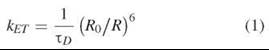
ΤD is the lifetime of the donor excited state in the absence of the acceptor; it is the average time an excited donor remains in the excited state (typical values of τD are between 1-10 ns). The rate of de-excitation of the donor in the absence of the acceptor is 1/TD. The constant R0 (see below) is defined as the distance R between the donor and acceptor molecules where the rate of transfer is equal to 1/TD. R0 is often approximately 5nm.
The rate of transfer shown in Equation 1 has an exceptionally strong 1/R6 distance dependence. As discussed above, the probability of energy transfer is in competition with all the other pathways of de-excitation. For instance, according to Equation 1, if the molecules are separated by less than about 0.5R0, then the rate of transfer is greater than 65 x (1/Td). Therefore, on the average, essentially all the excitation energy will be transferred from the donor to the acceptor. If the molecules are separated by 2R0 or greater, then the rate of transfer is less than 0.015 x (1/TD). Essentially, on the average, no energy will be transferred. Thus, as a rule of thumb, because often R0 ≈ 5 nm, FRET can only be used to determine distances less than 10 nm. For reasons that will be evident later, the lower limit is approximately 0.5 nm.
The constant R0 is dependent on several parameters: 1) the relative orientation of the transition dipole moments of the two molecules (these dipoles are the spectroscopic transition dipoles), 2) the extent that the fluorescence spectrum of the donor overlaps with the absorption spectrum of the acceptor, and 3) the surrounding index of refraction. We will deal with each of these below (see Equation 8). Because many proteins have diameters less than 10 nm, this distance dependence explains the usefulness of FRET for determining distances inside proteins as well as between interacting proteins, which is the reason that the name “spectroscopic ruler” was coined for FRET (20). FRET is a convenient method for determining the distance between two locations on proteins, or for determining whether two proteins interact intimately with each other. Fluorescence instrumentation is available in many laboratories, and a plethora of dyes and a wide variety of fluorescent proteins are now readily available. Therefore, FRET is a viable option for most researchers. With care, FRET can yield valuable information concerning protein-protein interactions, interactions of proteins with other molecules, and protein conformational changes.
Quantitative expressions for measuring the efficiency of FRET
The efficiency of FRET is the fraction of times that an excited donor molecule will transfer its excitation energy to an acceptor. For instance, if the efficiency of transfer is 0.3, and if a molecule is excited 100 times, then on average it will transfer the excitation energy to the acceptor 30 times. Another way to express the efficiency is by means of the rate of energy transfer (Eq. 1). After the donor has been excited from the ground state (S0) into its first excited singlet state (Si), the donor can exit the S1 state by several pathways (see Fig. 1a). As indicated in Fig. 1a, all pathways that lead away from the excited state of a chromophore (either to the ground state—by some radiative or nonradiative process—or passage to the triplet state) are in direct kinetic competition with each other. FRET is one of these pathways. Each ith pathway exits the excited state with a certain rate constant (ki in seconds-1). Figure 1b is a schematic that depicts the kinetic pathways. Because they are in direct competition, the probability of going by any single pathway (the efficiency of that pathway) is the ratio of the rate of that pathway divided by the sum of the rates of all the pathways. The efficiency of energy transfer, Fig. 2a, can be expressed as
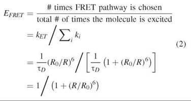
The k s are rate constants (with units of s-1), and the only ones that are included in Equation 2 are those that emanate directly out of the excited state of the donor (Fig. 1b). kET is the rate of undergoing FRET, ∑i ki is the sum of the rates over all the i th pathways (fluorescence emission, nonradiative de-excitation, quenching, photolysis, intersystem crossing to the triplet state, and including kEt), and EERET is the efficiency of energy transfer. The efficiency of fluorescence emission Efluor is defined analogously, and it is usually called the fluorescence quantum yield qem or фem. The efficiency can be defined this way for any of the pathways. It is also sometimes referred to as the quantum yield of the different pathways.
The lifetime of an excited molecule (in seconds) is the inverse of the sum of the kinetic rates (in s-1) for all the pathways for exiting the excited state. Thus in the absence of an acceptor, the lifetime is
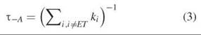
And in the presence of an acceptor, the lifetime is
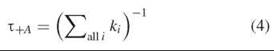
Therefore, the efficiency can also be given in terms of the measured fluorescence lifetimes in the presence and absence of an acceptor
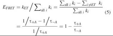
Thus one can determine the efficiency of FRET by measuring the nanosecond fluorescence lifetime of the donor in the presence (+A) and the absence (—A) of the acceptor. If one has the possibility of making this measurement, then it is a convenient, accurate, and robust way to measure the efficiency of FRET because the lifetimes can often be determined accurately, and not many corrections or experimental controls need to be made when calculating the efficiency.
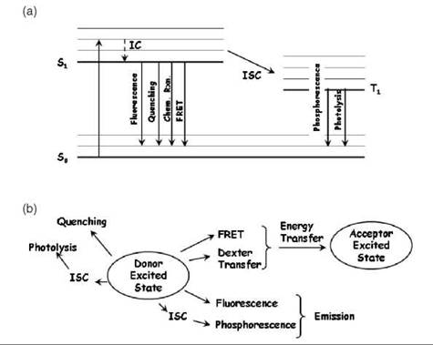
Figure 1. FRET and competing pathways. (a) A Perrin-Jablonski diagram shows common spectroscopic transitions for de-excitation of the donor fluorophore: Absorption of a photon excites the donor from the S0 to the S1 excited state, where it rapidly relaxes (typically in less than 1 ps) to the lowest vibrational level of the S1 state, which is known as internal conversion (IC). Internal conversion involves energy loss through vibrational interactions with the surroundings. The excited molecule in a higher vibrational state of S1 thereby releases heat to the surroundings, finally ending up in the lowest vibrational state of S1. The donor can then undergo de-excitation from the lowest vibrational level of the excited state to the S0 ground state through several pathways. The typical fluorescence lifetime (independent of the other pathways) is on order of 1-10 ns. Through spin-spin or spin-orbital interactions, the Si state can undergo intersystem crossing (ISC) into the excited triplet state where it spends some time (typically 10 n-s-10 s, depending on the concentration of oxygen in the solution) before phosphorescence or conversion to the ground state by internal conversion takes place. The ground state of oxygen is a triplet, and it can easily react with the triplet state of the chromophore, producing reactive oxygen species (radicals) that can collide with the chromophore, destroying it (photolysis). (b) This panel shows a schematic of the various competing pathways for leaving the excited donor state, including quenching, photolysis, fluorescence, and phosphorescence, which compete with FRET. Dexter transfer involves energy transfer to the acceptor molecule by exchange of electrons (see text) when the electronic orbitals of the donor and acceptor overlap. By measuring the effect of FRET on one of the competing processes (e.g., donor fluorescence), one can measure the FRET efficiency. It is not necessary to measure fluorescence to determine FRET efficiency, but this technique is the normal way. It is also possible to measure the fluorescence intensity of the acceptor (if the acceptor can fluoresce) to detect and quantify FRET (42, 48).
Several ways exist to determine the efficiency by measuring steady-state fluorescence. It is easily observed by inspecting the first equality in Equation 2. The best way to acquire steady-state values of the fluorescence intensity is photon counting. We will not go into the way it is done with hardware and electronics (it is usually done automatically with modern instrumentation), but simply note that by using photon counting one can easily measure a correct value of the intensity at any wavelength by counting the number of photons emitted. If one does not count photons, then the light detector must be corrected for the sensitivity of the photomultiplier at different wavelengths. We can rewrite Equation 2 as
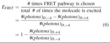
#(photons )D±A means the number of photons emitted by the donor in the presence or absence of the acceptor, respectively. This “counting” quantification is very important when measuring the efficiency of FRET, because the quantities of interest in Equation 6 are the number of photons emitted and the number of photons absorbed, and not their energy. The experiment can be conducted either on an ensemble of molecules (where different donor molecules will be excited by each excitation event) or by repetitive experiments on a single molecule. Thus, the numerator of Equation 6 is just the number of photons that the donor emits in the absence of an acceptor minus the number of photons emitted by the identical number (or concentration) of donors in the presence of an acceptor. This difference is just the number of “quanta” that are transferred to the acceptor, which would have been emitted as fluorescence photons if the acceptor were not there. The denominator is then simply the number of photons emitted by the donor in the absence of an acceptor. Thus, when the acceptor is far away, the efficiency is zero. When the acceptor is very close to the donor, the efficiency becomes one. Note the exact parallel of Equation 6 to Equation 5 (i.e., EFRET = 1 — T+A/T—A = 1 — #(photons)D.+A/#(photons)D.—A). This parallel relationship occurs because the lifetime of the donor emission becomes shorter when another pathway (for instance, kET) opens up for an escape from the excited state. That is, the average time in the excited state becomes shorter. It reduces the number of photons emitted by the donor by transferring a certain number of energy quanta from the excited donor to the acceptor. Often one measures the intensity of fluorescence. The intensity is proportional to #(photons )D.±A/second. Then, provided the concentration of the donor is the same in both measurements, and the conditions of measurement remain identical, the efficiency is
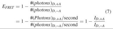
ID.±A is the measured fluorescence intensity of the donor in the presence and absence of the acceptor, which is measured under identical conditions and with the same donor concentration. If the concentration of the donor is not identical in both measurements, then it can usually be corrected simply by multiplying by the corresponding concentration ratio.
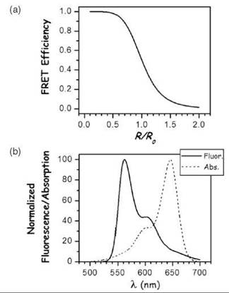
Figure 2. FRET characteristics. (a) The FRET efficiency as a function of R/RQ is shown E = 1/(1 + (R/R0)6). Proper selection of FRET pairs so that distances of interest lie near RQ where the FRET efficiency-distance slope is greatest will give the most sensitivity. (b) The spectral overlap requirement for FRET between the donor emission and the acceptor fluorescence spectrum is shown for the organic cyanine Cy3-Cy5 donor-acceptor pair.
Conditions for FRET and the Effect of the Transition Dipole Orientations
The value of R0 for a singular pair of D and A molecules is (1, 3, 6):
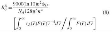
where, ![]() is wave number (in cm-1 units), фp is the quantum yield of the donor, NA is Avogadro’s number, n is the index of refraction pertaining to the transfer, εA(
is wave number (in cm-1 units), фp is the quantum yield of the donor, NA is Avogadro’s number, n is the index of refraction pertaining to the transfer, εA(![]() ) is the molar absorption coefficient of the acceptor (in units of cm-1mol-1), F(
) is the molar absorption coefficient of the acceptor (in units of cm-1mol-1), F(![]() ) is the fluorescence intensity of the measured fluorescence spectrum of the donor, and K2 is an orientation factor that results from the inner product between the unit vector of the electric near field of the donor dipole and the unit vector of the absorption transition dipole of the acceptor (see the Orientation Factor section below). The ratio of integrals in the bracket has units of cm6/mol. Using the units given in the paragraph above, we have:
) is the fluorescence intensity of the measured fluorescence spectrum of the donor, and K2 is an orientation factor that results from the inner product between the unit vector of the electric near field of the donor dipole and the unit vector of the absorption transition dipole of the acceptor (see the Orientation Factor section below). The ratio of integrals in the bracket has units of cm6/mol. Using the units given in the paragraph above, we have:
![]()
J(![]() ) is the ratio of integrals given in square brackets in Equation 8. We describe the parameters of this important equation below.
) is the ratio of integrals given in square brackets in Equation 8. We describe the parameters of this important equation below.
Distance dependence
For energy to be transferred from the donor to the acceptor, an interaction must occur between the two molecules, and the energy must be conserved (i.e., the energy lost by the donor equals that gained by the acceptor). Coulomb (charge-charge) interactions between the electron distributions in both molecules are responsible for the FRET interaction, and the energy transfer can be understood as an interaction between two classical oscillating dipoles. Actually, a classical derivation of the FRET equations (87, 26) results in the identical expression as a quantum mechanical derivation (3, 48). The electric field of an oscillating dipole is very large in the “near-field” region where the field can be described by a pure dipole field (Fig. 3a). A dipole field at some point in space a distance R from the center of the dipole is dependent on the angle relative to the dipole direction, and it varies with distance as 1/R3. The interaction energy between the two dipoles therefore varies as 1/R6. The interaction energy also depends on the relative orientations of the two dipoles and the orientation of each dipole to the separation vector between the two dipoles (see Figs. 3a and 3b). The dipole-dipole nature of the interaction explains the 1/R6 dependence of the rate of energy transfer (Eq. 1).
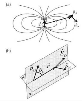
Figure 3. The electric field of the donor and the orientation factor. (a) The acceptor dipole ![]() in the electric field
in the electric field ![]() of the donor
of the donor ![]() is the distance between the point dipoles. ΘD is the angle between
is the distance between the point dipoles. ΘD is the angle between ![]() and
and![]() (b) This schematic shows the donor and acceptor dipoles and illustrates the angles and radial vectors used in the definition of the orientation factor k2. The coordinate system is chosen such that the
(b) This schematic shows the donor and acceptor dipoles and illustrates the angles and radial vectors used in the definition of the orientation factor k2. The coordinate system is chosen such that the ![]() and
and ![]() vectors are in the r-y plane; the
vectors are in the r-y plane; the ![]() vector can be in any direction, and is not supposed to be in either the r-y or r-x planes. The dipole field is symmetrical about the azimuthal angle of the
vector can be in any direction, and is not supposed to be in either the r-y or r-x planes. The dipole field is symmetrical about the azimuthal angle of the ![]() vector.
vector.
Overlap integral
It is important to realize that in this near-field zone of the dipoles (which extends maximally 10 nm for FRET) no photon exists; the lack of photons in the near-field zone is essentially because of the Heisenberg uncertainty principle of quantum mechanics (88). That is, the energy is transferred without the emission or absorption of a photon. Of course, the energy transferred from the donor must equal exactly the energy transferred to the acceptor. However, it turns out that the interaction between the two molecules in the near-field zone can be described as if the acceptor is bathed in an oscillating electric field of the near-field zone of the donor, ![]() in Equation 10. This oscillating electric field (with a frequency equal to that of the fluorescence of the donor emission, F(
in Equation 10. This oscillating electric field (with a frequency equal to that of the fluorescence of the donor emission, F(![]() ) of Equation 8) is in the near-field zone of the donor where no photons exist and not in the far field zone where photons exist. The energy of such a Hertzian oscillating dipole is not emitted as photons until a distance of about one wavelength away from the donor. Energy is conserved during the transfer event; that is, the energy lost by the donor must equal the energy taken up by the acceptor. The change in the energy levels of the donor and the acceptor are the same energy levels that correspond to the spectroscopic transitions of the donor (the emission spectrum) and acceptor (the absorption spectrum). Therefore, to conserve energy, the emission (fluorescence) spectrum of the donor F(
) of Equation 8) is in the near-field zone of the donor where no photons exist and not in the far field zone where photons exist. The energy of such a Hertzian oscillating dipole is not emitted as photons until a distance of about one wavelength away from the donor. Energy is conserved during the transfer event; that is, the energy lost by the donor must equal the energy taken up by the acceptor. The change in the energy levels of the donor and the acceptor are the same energy levels that correspond to the spectroscopic transitions of the donor (the emission spectrum) and acceptor (the absorption spectrum). Therefore, to conserve energy, the emission (fluorescence) spectrum of the donor F(![]() ) must overlap with the excitation (absorption) spectrum εA(
) must overlap with the excitation (absorption) spectrum εA(![]() ) of the acceptor (Fig. 2b). The more these spectra overlap, the stronger is the energy transfer; that is, a larger spectral overlap leads to a longer R0. The F(
) of the acceptor (Fig. 2b). The more these spectra overlap, the stronger is the energy transfer; that is, a larger spectral overlap leads to a longer R0. The F(![]() ) and εA(
) and εA(![]() ) spectra (Fig. 2b) are those of the separate donor and acceptor components. These spectra must be the appropriate spectra that correspond to the identical conditions as where the FRET measurements are made. Often the spectra can simply be taken from the literature that refers to the separate dyes. But often, the dyes physically interact with the proteins, which changes the dyes’ absorption or emission spectra. The overlap integral involves the weighting function
) spectra (Fig. 2b) are those of the separate donor and acceptor components. These spectra must be the appropriate spectra that correspond to the identical conditions as where the FRET measurements are made. Often the spectra can simply be taken from the literature that refers to the separate dyes. But often, the dyes physically interact with the proteins, which changes the dyes’ absorption or emission spectra. The overlap integral involves the weighting function ![]() -4 in addition to the emission spectrum of the donor and the absorption spectrum of the emitter (see Eq. 8).
-4 in addition to the emission spectrum of the donor and the absorption spectrum of the emitter (see Eq. 8).
As mentioned above, although no photon is emitted or absorbed in the transfer process, the emission spectrum of the donor and the absorption spectrum of the acceptor are still involved in the overlap integral. This participation of the optical spectra is because FRET involves changes in the energy levels of D and A that are identical to those in normal absorption and emission events. An important condition for Forster transfer is that the interaction between the donor and acceptor is very weak, and the two molecular species retain their separate electronic and vibrational structures and energy levels. In FRET, the donor and acceptor are very weakly perturbed by dipole interactions, which is formally the same type and strength of interaction that describes the interaction of the chromophores with light. Therefore, the energy transitions, which can occur in the donor and acceptor molecules during FRET, are the same as their respective spectroscopic transitions when absorbing or emitting photons. This requirement for the conservation of energy, which is expressed by the overlap integral in the expression for R0 (Eqs. 8 and 9), is also the reason for the word “resonance” in FRET. We emphasize once more: Although the emission and absorption spectra of the donor and acceptor are in the overlap integral, the FRET process does not involve the emission or the absorption of a “photon.” The quantum of energy transferred by FRET takes place in the near field of the oscillating dipoles (quantum mechanically the transition dipoles), where the energy cannot yet be described in terms of real photons.
Orientation factor K2
The parameter K2 in Equation 8 is referred to as the orientation factor of FRET. This factor represents the angular dependence of the interaction energy between the acceptor transition dipole and the oscillating dipole electric field of the donor. K2 is the source of much debate and many misunderstandings. It is the most difficult factor to control and usually the hardest to determine with confidence (28, 48). Therefore, we will spend more time discussing this factor.
To understand this angular dependence of the acceptor transition dipole in the donor electric field, we first express the electric dipolar interaction between the donor and acceptor molecules classically. The energy of interaction between the donor and acceptor dipoles is directly proportional to the vector dot product of the electric field of the donor with the dipole moment of the acceptor. The equations for FRET have been derived classically (87, 26, 48) by assuming that the donor molecule is an oscillating point dipole [a Hertzian dipole (89)]. One assumes that the acceptor is located in the “near-field zone” (which extends much less than one wavelength of light of the corresponding frequency) of the oscillating dipole of the donor (Fig. 3). The acceptor absorbs the energy by interacting with the oscillating near field of the donor (the donor oscillates at the same optical frequency where the acceptor absorbs). The near field is not radiating (no transverse photon emission occurs in the near-field zone of a Hertzian dipole). And the electric field in the near field has both longitudinal and transverse components, in contrast to the far field zone, where the electric field has only transverse components. Nevertheless, the mechanism of absorption of energy by the acceptor from the oscillating electric field of the donor Hertzian dipole is identical to the mechanism of absorption of light of the same frequency. Therefore, the interaction of the “transition moment” of the acceptor with the electric field of the donor obeys the same rules as normal absorption of light by the acceptor (polarization dependence and all the spectral requirements for normal absorption). The rate of absorption is proportional to the square of the vector dot product of the acceptor transition dipole with the electric field of the donor, just as though this field were equivalent to the oscillating electric field of light impinging on the acceptor. However, the electric field in the near-field of the donor is not propagating, and the field direction has longitudinal as well as transverse vector components [propagating light (photons) has only vector components transverse to the direction of propagation]. This electric field is a reflection of the fact that in the near-field zone no photon could even exist according to the uncertainty principle. This simple classical description (which results in the correct theoretical description of FRET) is also perfectly consistent with a quantum derivation.
The orientation factor can be best understood quantitatively by studying the interaction of the acceptor dipole in the near-field zone of the donor (Fig. 3a). The energy of interaction of the donor electric field ED, and the acceptor dipole moment ![]() , is
, is ![]() ∙
∙ ![]() . The rate of absorption is proportional to the square of this energy of interaction. "Therefore, the rate of energy transfer is proportional to (
. The rate of absorption is proportional to the square of this energy of interaction. "Therefore, the rate of energy transfer is proportional to (![]() ∙
∙ ![]() )2 (Eq. 11).
)2 (Eq. 11).
The field ![]() that surrounds an oscillating classical electric dipole
that surrounds an oscillating classical electric dipole ![]() is shown in Fig. 3a,
is shown in Fig. 3a,
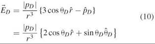
where |pD| is the time independent dipole strength, r = |![]() | is the distance from the point donor dipole (in FRET it is the distance from D to A), and
| is the distance from the point donor dipole (in FRET it is the distance from D to A), and ![]() is the unit vector pointing from the donor dipole to the position
is the unit vector pointing from the donor dipole to the position ![]() , where the acceptor is located. θD is the polar angle between
, where the acceptor is located. θD is the polar angle between ![]() and
and ![]() .
. ![]() is a unit vector perpendicular to r that points in the direction of increasing θD (Fig. 3a). The caps designate unit vectors. Figure 3b shows the juxtaposition of two dipoles, and it defines the parameters used in the Equations 10, 11, and 12. As we said above, kET in Equation 1 is proportional to (
is a unit vector perpendicular to r that points in the direction of increasing θD (Fig. 3a). The caps designate unit vectors. Figure 3b shows the juxtaposition of two dipoles, and it defines the parameters used in the Equations 10, 11, and 12. As we said above, kET in Equation 1 is proportional to (![]() ∙
∙ ![]() )2, according to classic electrodynamics. We can write
)2, according to classic electrodynamics. We can write
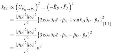
where K2 has been defined as
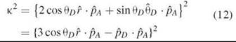
![]() The orientation factor K2 can have values between 0 and 4. We have given K2 in two different representations in Equation 12.
The orientation factor K2 can have values between 0 and 4. We have given K2 in two different representations in Equation 12.
Thus, the rate of energy transfer depends on the square of the dot product between the acceptor dipole (transition dipole) ![]() and the field
and the field ![]() of the donor dipole (transition dipole),
of the donor dipole (transition dipole), ![]() (Eq. 11 and Fig. 3b). For any chosen locations and orientations of the donor and acceptor, the value of K2 involves the cosine of the angle between the unit vectors
(Eq. 11 and Fig. 3b). For any chosen locations and orientations of the donor and acceptor, the value of K2 involves the cosine of the angle between the unit vectors ![]() and
and ![]() (i.e.,
(i.e., ![]() ∙
∙ ![]() ) as well as the cosine of the angles between r and pA (i.e.,
) as well as the cosine of the angles between r and pA (i.e., ![]() ∙
∙ ![]() ) and between
) and between ![]() and
and ![]() (i.e.,
(i.e., ![]() ∙
∙ ![]() ). Therefore, for any constant selected angle between the donor and acceptor dipoles (that is, constant
). Therefore, for any constant selected angle between the donor and acceptor dipoles (that is, constant ![]() ∙
∙ ![]() ), the value of K2 will depend on the position in space where the acceptor dipole is relative to the donor. The strength of the field of the donor molecule for any particular constant values of θD, θA and
), the value of K2 will depend on the position in space where the acceptor dipole is relative to the donor. The strength of the field of the donor molecule for any particular constant values of θD, θA and ![]() ∙
∙![]() changes with the distance |
changes with the distance |![]() | as 1/r3, that is, for any particular direction of
| as 1/r3, that is, for any particular direction of ![]() relative to
relative to ![]() . As illustrated in Fig. 3a, for a particular angle between the orientations of the donor and acceptor dipoles (
. As illustrated in Fig. 3a, for a particular angle between the orientations of the donor and acceptor dipoles (![]() ∙
∙ ![]() ), the angle between the acceptor dipole and the electric field of the donor depends on the position in space of the acceptor. Also, for constant relative orientations of the donor and acceptor dipoles (constant
), the angle between the acceptor dipole and the electric field of the donor depends on the position in space of the acceptor. Also, for constant relative orientations of the donor and acceptor dipoles (constant ![]() ∙
∙ ![]() ), and for constant cos θD
), and for constant cos θD![]() ∙
∙ ![]() , K2 is constant (Eq. 11 and 12). In this case, the rate of FRET is solely a function of the distance between the donor and acceptor. However, if only
, K2 is constant (Eq. 11 and 12). In this case, the rate of FRET is solely a function of the distance between the donor and acceptor. However, if only ![]() ∙
∙ ![]() and θD are constant, then the distance dependence is more complicated than just the distance between the donor and acceptor. This intertwining relationship between the distance separating the donor and acceptor and the orientational dependence of K2 illustrates the complexity of determining a value for K2.
and θD are constant, then the distance dependence is more complicated than just the distance between the donor and acceptor. This intertwining relationship between the distance separating the donor and acceptor and the orientational dependence of K2 illustrates the complexity of determining a value for K2.
Because the orientations and spatial locations of the two chromophores may vary over the ensemble of molecules, and because they can also change during the time the donor is in the excited state, the measured effect of K2 is usually an average over the appropriate spatial/temporal distributions. Whenever ![]() and the acceptor dipole moment
and the acceptor dipole moment ![]() have parallel orientations, the rate of FRET is maximum for that placement in space for the acceptor relative to the donor. For
have parallel orientations, the rate of FRET is maximum for that placement in space for the acceptor relative to the donor. For ![]() oriented parallel to
oriented parallel to ![]() , the possible maximum values of K2 are between 1 and 4; that is, the actual maximum value depends on the value of θD (see below). The minimum value of K2 is zero for every position of the acceptor relative to the donor whenever ED and the acceptor dipole moment
, the possible maximum values of K2 are between 1 and 4; that is, the actual maximum value depends on the value of θD (see below). The minimum value of K2 is zero for every position of the acceptor relative to the donor whenever ED and the acceptor dipole moment ![]() are oriented perpendicular to each other.
are oriented perpendicular to each other.
The possible introduction of error in the estimation of the FRET efficiency from the orientation factor is often of concern when measuring FRET in proteins or between proteins. This uncertainty can occur because the actual distribution of dye orientations is often not known, or because the dyes do not rotate freely and rapidly relative to the fluorescence lifetime of the donor. If the donor and acceptor molecules undergo rotational or translational movements during the time the donor is in the excited state, or if an ensemble of different donor and acceptor orientations exist, then the value ofK2 (and of course the rate) will be averaged over the corresponding ensemble of configurations. Because K2 can, in principle, range from 0 (e.g., acceptor absorption dipole perpendicular to the electric field of the donor) to 4 (e.g., end-to-end stacked parallel dipoles), the variation in the rate of FRET can be extensive because of such movements. This possible variation in K2 becomes especially apparent when one notes that the measurement of the rate of transfer (or the efficiency) varies directly as R06, and therefore directly with K2 (see below). If the condition of very rapid (compared with the lifetime of the donor) rotational movements of both donor and acceptor is met, then K2 is rigorously 2/3, which arises from averaging over all possible orientations. If rapid re-orientation through all angles is not the case, then limitations on the degree of rotational freedom can have significant effects on the measured efficiency of energy transfer. However, as we discuss below, the assumption thatK2 = 2/3 is often a justified, and reasonable one to make (39, 48, 86).
It is worthwhile to consider a few simple examples to get a feeling for the values of K2. If the two dipoles have orientations in space perpendicular to each other, and if the acceptor dipole is juxtaposed next to the donor, but in the direction perpendicular to the direction of the donor dipole, then K2 = 0 (that is, because, θD = π/2, so cos θD = 0, and ![]() ). However, this example is only a special case where K2 = 0. As was pointed out above, for any position in space of the acceptor molecule, K2 will equal zero for all orientations of
). However, this example is only a special case where K2 = 0. As was pointed out above, for any position in space of the acceptor molecule, K2 will equal zero for all orientations of ![]() where
where ![]() And for most of these positions where
And for most of these positions where ![]() , the donor and acceptor dipoles are not perpendicular to each other (see Fig. 3a). Conversely, if the donor and acceptor dipoles are perpendicular, then most locations of the acceptor relative to the donor will have K2 ≠ 0. This relationship is easiest to observe by looking at the second equality in Equation 12 or by examining Fig. 3a. Another simple example is when the dipoles are parallel
, the donor and acceptor dipoles are not perpendicular to each other (see Fig. 3a). Conversely, if the donor and acceptor dipoles are perpendicular, then most locations of the acceptor relative to the donor will have K2 ≠ 0. This relationship is easiest to observe by looking at the second equality in Equation 12 or by examining Fig. 3a. Another simple example is when the dipoles are parallel ![]() Then, if θD = 0 and
Then, if θD = 0 and ![]() (parallel dipoles, stacked on each other), then K2 = 4. But when θD = π/2 and
(parallel dipoles, stacked on each other), then K2 = 4. But when θD = π/2 and ![]() (again parallel dipoles, but now next to each other), then K2 = 1. In the latter case,
(again parallel dipoles, but now next to each other), then K2 = 1. In the latter case, ![]() is parallel to
is parallel to ![]() but
but ![]() and the value of K2 is four times smaller than when cos
and the value of K2 is four times smaller than when cos ![]() These few examples demonstrate the complexity of the behavior of K2. In Fig. 3a, we have indicated both the orientation of
These few examples demonstrate the complexity of the behavior of K2. In Fig. 3a, we have indicated both the orientation of ![]() and
and ![]() as well as the angle θD (where cos
as well as the angle θD (where cos ![]() ). More thorough discussions of kappa can be found in the literature (35, 48, 51).
). More thorough discussions of kappa can be found in the literature (35, 48, 51).
Because fluctuations always exist in positions and angles of the D and A molecules, the actual value of K2 is an ensemble average or a time average. The most commonly used average value is K2 = 2/3. As already mentioned, this result is rigorously true if during the excited state lifetime of the donor the orientations of the donor and acceptor can each individually reorient fully in an independent random fashion. However, even when this condition is not met (for instance when the anisotropy of the dyes is not close to zero), it has been found that the approximation K2 = 2/3 is often satisfactory (39, 42, 45, 51, 90). It is often discussed in the literature as though K2 = 2/3 pertains only to the case of very rapidly rotating D and A molecules. This statement is not true, because depending on the placement of the dyes and their relative orientations, it is possible for K2 = 2/3 at every location of the acceptor relative to the donor, even when the dyes cannot rotate at all. Also, many dyes used for FRET have more than a single transition dipole, which can be excited at the same wavelengths. Because different transition dipoles of a fluorophore are usually not parallel to each other (they are often perpendicular to each other), the presence of multiple transition dipoles leads again to an averaging of K2 (90).
Finally, if one is interested in detecting a change in structure or extent of interaction (binding), then one may not be interested in exact estimates of K2. For instance, when fluorescent proteins are used in FRET experiments, K2 can become a very important variable, and averages are often not applicable. This situation occurs because the chromophores are fairly rigidly held in the fluorescent protein structure, and the fluorescent proteins may have specific interactions either with each other or with other components of the complex under study (91, 92).
Index of refraction
Note that in Equations 8 and 9, R06 α 1/n4, which means that the distance over which FRET can take place is shortened for higher indices of refraction in the molecular surroundings (the solvent). A high index of refraction—which is equal to the square root of the dielectric constant—means that the electrons in the molecules of the solvent are freer to respond to an electric field than for solvents with lower indices of refraction. The solvent is assumed not to absorb at the wavelengths in question, so the index of refraction is real (not a complex number). This screening from the response of the solvent molecules leads to a damping of the extent of the field, and therefore the two dipoles (donor and acceptor) must be closer together in a solvent with higher index of refraction to have the same strength of interaction as in a solvent with lower index of refraction. Note that the wavelengths are also shorter in a higher index of refraction; however, remember that FRET does not involve propagating light fields. The actual situation is somewhat more complex, and the reader is referred to an excellent discussion in the recent literature (93-95), which clears up common misconceptions as to the origin of the effect of the index of refraction for FRET. In addition, the index of refraction varies significantly over short distances in and on the surface of proteins (90); for very short distances, the concept of an index of refraction becomes suspect. However, usually an average value is chosen between 1.33 and 1.5, which correspond to values of water and crystals of polypeptides. The value chosen usually depends on whether the dyes are in direct contact with water or are inside the protein, where the dyes are removed from water. Detailed numerical methods (96, 76, 97, 70) can be used to take into account directly the interaction between charges if the protein structures are known and if the position and orientations of the chromophores are known. Such extensive numerical calculations, whenever the structures are well known, avoid the use of an “effective” index of refraction.
Quantum yield of the donor
Equation 8 shows that R0 is dependent on the quantum yield of the donor фD. This dependence is not strong; R0 α (фD)1/6. For instance, ![]() Therefore, small changes in the quantum yield of the donor will not make large differences in the value of R0. Of course, if increasing §D by a factor allows one to make accurate measurements of distances or to observe conformational changes, then the change can be significant. However, the range of distances observable by FRET are not a strong function of the quantum yield of the donor. However, small displacements in the horizontal placement of the efficiency curve of Fig. 2a can significantly increase or decrease the sensitivity of a FRET measurement. In some circumstances, it is advisable to choose a donor-acceptor pair that have a smaller R0, preferably in the range of the distance one is interested in measuring (see section below on “What is important, R06 or R0?”). One can sometimes shorten R0 by simply adding a collisional dynamic quencher to the solution, which will lower the quantum yield of the donor in the absence of the acceptor, lowering TD , thereby adjusting R0 to lower values (90).
Therefore, small changes in the quantum yield of the donor will not make large differences in the value of R0. Of course, if increasing §D by a factor allows one to make accurate measurements of distances or to observe conformational changes, then the change can be significant. However, the range of distances observable by FRET are not a strong function of the quantum yield of the donor. However, small displacements in the horizontal placement of the efficiency curve of Fig. 2a can significantly increase or decrease the sensitivity of a FRET measurement. In some circumstances, it is advisable to choose a donor-acceptor pair that have a smaller R0, preferably in the range of the distance one is interested in measuring (see section below on “What is important, R06 or R0?”). One can sometimes shorten R0 by simply adding a collisional dynamic quencher to the solution, which will lower the quantum yield of the donor in the absence of the acceptor, lowering TD , thereby adjusting R0 to lower values (90).
Transfer at very short distances
The Förster transfer mechanism (Eqs. 1, 8, and 10) is valid at all distances in the near-field region where the approximation of point dipoles is valid. At very small distances from the molecular dipoles, the finite extended distribution of the electrons make the point dipole approximation invalid (98, 99). In this case, the higher order terms such as quadrapoles and octapoles would have to be taken into account (14, 15). In addition, if no electric dipole interactions occur between the donor and acceptor (for symmetry conditions, making the transition dipole zero), then these electric quadrapole terms and interactions between the magnetic dipole and electric dipole terms have to be taken into account. The lack of electric dipole transitions is seldom the case, and the use of quadrapole terms has not yet been important for the interpretation of FRET in proteins. However, if the two participating dipoles are very close, then transfer by electron exchange [Dexter transfer (14, 15)] also presents a possible pathway for energy transfer. This type of energy transfer should not be referred to as FRET because it is a different mechanism than Forster Transfer and requires a partial overlap of the electronic orbitals of the donor and acceptor. The transfer probability drops off exponentially, following the exponential decrease in the overlap of the wave functions of the electronic orbitals. However, even in photosynthesis, where the chlorophylls are very close and oriented to maximize energy transfer, it has not been shown unequivocally whether Dexter transfer is an important pathway for energy transfer in the photosynthetic unit. Nevertheless, one should be aware of these other mechanisms of energy transfer.
Noncoherent energy transfer (FRET) or coherent transfer
Lately there has been increased interest in coherent transfer. Forster transfer assumes that interactions with the molecular surroundings, or the internal vibrations of the molecules, are sufficiently rapid so no correlation exists between the act of excitation of the donor and the act of transfer. In other words (to give an anthropomorphic analogy), during the time when FRET can take place the donor shows no memory of how, or when, it was excited. This lack of memory is attributed to the chaotic, randomizing effects take place in subpicosecond times, rapidly relaxing the initially excited molecule to the lowest vibrational state of the excited electronic state (before fluorescence emission or FRET). A similar process takes place after the energy is transferred to the acceptor; the original acceptor state immediately following the transfer is rapidly randomized so that the transfer is irreversible. Whenever this randomization occurs, energy transfer can be analyzed from a probability viewpoint (Forster transfer), as is the case in the derivation of the Equations 2-7, 8, and 11. That is, in Forster transfer we consider the probability per unit time for each pathway where the probabilities are independent of time and independent of each other. This probabilistic treatment of all the rates of deexcitation from the excited state for Forster transfer holds true whether the donor and acceptor are identical (homo-FRET) or different molecules (hetero-FRET). If molecules (or atoms, with which most of these coherent transfer experiments have taken place) are completely isolated from the environment (such as in a vacuum at very low temperatures, e.g. well below 1 K), or if one is observing the fluorescence emission in the femtosecond time range at low temperatures (<77 K), then it is possible to observe coherent transfer. Under the right conditions, the energy oscillates between different states (with the energy localized on different molecules or atoms) as a function of time; that is, the location of the excitation energy is not localized on just one chromophore independent of time. Instead, the energy is distributed between different chromophores and oscillates from one to the other. These oscillations can be observed in the time dependence of the fluorescence emission. Analogous oscillations in the transfer of energy between different interacting molecules in resonance (even without emission) were first described by Schrodinger (100). Until recently, it was not considered relevant for protein systems; however, lately these oscillations have been observed for photosynthetic systems at low temperatures (101,102). How important these coherent oscillations are for the mechanism of photosynthesis at normal temperatures remains to be determined. But the effect has created much interest. The question is whether this coherent transfer, which is very rapid and can therefore transfer energy over large distances before the processes that lead to transfer becomes incoherent, plays a major role in the efficiency of photosynthesis.
What is Important: R06 or R0, and When?
Whether R06 or R0 are more important, may sound like a silly question; however, a subtle difference determines when one may be of more interest than the other. Usually, R0 is stressed. R0 is the distance where the rate of transfer is half the rate of de-excitation from the excited state (1/TD in Eq. 1). One usually tries to choose dye pairs (donor and acceptor) such that the expected range of R is in the most sensitive part of the efficiency curve (Fig. 2a). Choosing appropriate donor and acceptor molecules can be done by trial and error, researching the literature, or determining the variable parameters in Equation 8 and calculating R0. The variable experimental parameters that define Ro are![]() n, K2, and фD. To make calculations of R0, one usually chooses K2 = 2/3, and then corrects the K2 = 2/3-calculated R0 by the appropriate factor if it is suspected that K2 = 2/3. Because R0 is proportional to the 1/6 power of
n, K2, and фD. To make calculations of R0, one usually chooses K2 = 2/3, and then corrects the K2 = 2/3-calculated R0 by the appropriate factor if it is suspected that K2 = 2/3. Because R0 is proportional to the 1/6 power of ![]() K2 and фD, the value of R0 is not a strong function of these parameters; therefore, variations in their values do not change the value of R0 very much. As we pointed out above, R0 is proportional to the 4/6 power of the index of refraction, n. So a fractional change in the index of refraction can have a more significant effect on R0. For instance, a 20% change in K2 will change R0 by only 3%. However, a 20% change in n will change R0 by 13%. So, all the variations in R0 are smaller than the corresponding variation in the parameter itself. Even if the parameters change by a factor of 2 (except for n), R0 will only change by 12%, which is the reason that the R0 of many dyes are in the same range. So, one might get the idea that variations in these parameters will be insignificant compared with the expected (or searched for) changes in distance.
K2 and фD, the value of R0 is not a strong function of these parameters; therefore, variations in their values do not change the value of R0 very much. As we pointed out above, R0 is proportional to the 4/6 power of the index of refraction, n. So a fractional change in the index of refraction can have a more significant effect on R0. For instance, a 20% change in K2 will change R0 by only 3%. However, a 20% change in n will change R0 by 13%. So, all the variations in R0 are smaller than the corresponding variation in the parameter itself. Even if the parameters change by a factor of 2 (except for n), R0 will only change by 12%, which is the reason that the R0 of many dyes are in the same range. So, one might get the idea that variations in these parameters will be insignificant compared with the expected (or searched for) changes in distance.
However, the measured variation in the rate of transfer (Eq. 1) is proportional to R06, which means that variations these parameters could have a much more significant effect on the measured efficiency. If R is not approximately within R0 ± 0.5 R0, then the measured efficiency (Eq. 2) will not depend on variations or changes in these parameters significantly (Fig. 2a), because the efficiency is within about 8% of the minimum or maximum value, and such small changes may be hard to measure. However, if one is in the range R = R0 ± 0.5R0, then the changes in any of the parameters ![]() n, K2 and фD can lead to significant changes in the efficiency that could be confused with changes in R. The sensitivity to such conformational changes (if the dyes are chosen with judicious values of R0) is one of the valuable characteristics of FRET. This possibility should be carefully considered, especially whenever one is using FRET to measure changes in protein structure and wants to interpret the results as a change in R (see, for instance Reference 90). In any case, as is clear from looking at Equation 1, one achieves maximum efficiency for observing small changes in D—A distances when R is approximately equal to R0. The take-home message is that when choosing dyes for specific cases, it is worthwhile to consider carefully the choice of dyes, investigate their spectroscopic properties, and calculate the R0. It is not necessarily the best choice to select dye pairs that show the maximum values of R0.
n, K2 and фD can lead to significant changes in the efficiency that could be confused with changes in R. The sensitivity to such conformational changes (if the dyes are chosen with judicious values of R0) is one of the valuable characteristics of FRET. This possibility should be carefully considered, especially whenever one is using FRET to measure changes in protein structure and wants to interpret the results as a change in R (see, for instance Reference 90). In any case, as is clear from looking at Equation 1, one achieves maximum efficiency for observing small changes in D—A distances when R is approximately equal to R0. The take-home message is that when choosing dyes for specific cases, it is worthwhile to consider carefully the choice of dyes, investigate their spectroscopic properties, and calculate the R0. It is not necessarily the best choice to select dye pairs that show the maximum values of R0.
Examples of FRET and Proteins
For over 50 years, FRET has been applied to protein and peptide structures (16, 34). It would be impossible to review even a small selection of the vast literature, and the following list of applications does not attempt to present details of the methodologies or the results. We will present just a few selected publications to give a flavor of the type of problems where FRET is applied, and from which the interested reader can obtain references.
FRET has been shown to acquire reliable estimates of protein and other macromolecular structures (27, 34, 53, 90, 103-108). Attention must be paid to the relative orientations of the transition dipoles of the donor and acceptor (28), but it has also been shown that for many biological systems, the approximation K2 = 2/3 is reasonable and gives correct distances despite relatively high fluorescence anisotropies of the donor and/or acceptor emissions (39, 109, 90). Reasons for this approximation have been discussed (48). Conformational changes based on singular positions of the donors and acceptors as well as donor-acceptor distributions can be observed (110-112). Dynamics of protein conformational changes can be observed in the nanosecond time range by measuring the fluorescence lifetimes of the donor or by following steady-state fluorescence of the donor or acceptor at longer times (110, 113-117). FRET is also very useful as the measurement basis of biochemical assays (118). The stoichiometry and formation of macromolecular assemblies and aggregated protein structures can often be quantified by well-planned and correctly analyzed FRET measurements (119-124). A common problem in FRET studies can occur with the use of multi-donors and multi-acceptors. But analysis methods have been developed to take this problem into account, and it can also be an advantage when determining structures (125-127).
FRET has been widely used to determine the distribution of proteins in membranes and their interactions in two dimensional systems, as well to detect communication across membranes (128-137).
The introduction of fluorescent proteins have been a great addition to the repertoire of FRET measurements of protein systems in solution and especially in fluorescence microscopy (138-141). Indeed, the number of applications of FRET in fluorescence microscopy have exploded in recent years, and novel analysis methods have also been developed in order to extract quantitative parameters from image data (142-146).
In bioluminescence resonance energy transfer (BRET), the excitation of the donor is carried out with a biological/chemical reaction instead of light excitation. It was discovered as a naturally occurring phenomenon (147). The photoprotein aequorin in Aequorea emits blue light when alone; however, when GFP and aequorin are associated in vivo, GFP accepts the energy from aequorin and emits green light. The use of bioluminescence as a donor in vitro was realized early (148), and it has undergone a renaissance because of the availability of the biological systems used for donor and acceptor excitation (149, 150). In general, the donor is replaced by luciferase, which becomes excited chemically in the presence of a substrate and can transfer its energy to an acceptor, which is usually (although not necessarily) a fluorescent protein (149, 150). BRET is very useful in microscopy and the background fluorescence is essentially zero. BRET has also been used in high-throughput screening (151).
References
1. Forster T. Energiewanderung und Fluoreszenz. Naturwissens- chaften 1946; 6:166-175.
2. Forster T. Fluoreszenzversuche an Farbstoffmischungen. Angew Chem. A 1947; 59:181-187.
3. Forster T. Zwischenmolekulare Energiewanderung und Fluoreszenz. Ann. Phys. 1948; 2:55-75.
4. Forster T. Expermentelle und theoretische untersuchung des zwischengmolekularen ubergangs von elektronenanregungsenergie. A Naturforsch. 1949; 4A:321-327.
5. Forster T. Versuche zum zwischenmolekularen ubergang von elektronenanregungsenergie. Z Elektrochem. 1949; 53:93-100.
6. Forster T. Fluoreszenz Organischer Verbindungen. 1951. Vandenhoeck & Ruprecht, Gottingen. pp. 315.
7. Forster T. Transfer mechanisms of electronic excitation. Discuss Faraday Soc. 1959; 27:7-17.
8. Forster T. Transfer mechanisms of electronic excitation energy. Radiat. Res. Suppl. 1960; 2:326-339.
9. Forster T. Delocalized excitation and excitation transfer. In: Modern Quantum Chemistry; Part III; Action of Light and Organic Molecules. Sunanoglu O. eds. 1965. Academic Press, New York. pp. 93-137.
10. Forster T. Intermolecular energy migration and fluorescence. In: Biological Physics. Mielczarek EV, Greenbaum E, Knox RS, eds. 1993. Americal Institute of Physics, New York. pp. 148-160.
11. Perrin J. Fluorescence et induction moleculaire par resonance. C.R. Hebd. Seances Acad. Sci. 1927;184:1097-1100.
12. Perrin F. Theorie quantique des transferts d’activation entre molecules de meme espece. Cas des solutions fluorescentes. Ann. Chim. Phys. 1932; 17:283-314.
13. Perrin F. Interaction entre atomes normal et activite. Transferts d’activitation. Formation d’une molecule activitee. Ann. Institut Poincare. 1933; 3:279-318.
14. Dexter D. A theory of sensitized luminescence in solids. J. Chem. Phys. 1953; 21:836-850.
15. Dexter DL, Schulman JH. Theory of concentration quenching in inorganic phosphores. J. Chem. Phys. 1954; 22:1063-1070.
16. Stryer L. Energy transfer in proteins and polypeptides. Radiat. Res. 1960; (2):432-451.
17. Bennett G, Schwekmer R, Kellogg R. Radiationless intermolecular energy transfer. II. Triplet-singlet transfer. J. Chem. Phys. 1964; 41:3040-3041.
18. Bennett R. Radiationless intermolecular energy transfer. I. Singlet-singlet transfer. J. Chem. Phys. 1964; 41:3037-3040.
19. Bennett G, Kellogg R. Mechanisms and rates of radiationless energy transfer. Prog. React. Kinet. 1967; 4:215-238.
20. Stryer L, Haugland R. Energy transfer: A spectroscopic ruler. Proc. Natl. Acad. Sci. U.S.A. 1967; 58:719-726.
21. Steinberg I. Nonradiative energy transfer in systems in which rotatory Brownian motion is frozen. J. Chem. Phys. 1968; 48:2411-2413.
22. Steinberg I, Katchalski E. Theoretical analysis of the role of diffusion in chemical reactions, fluorescence quenching, and nonradiative energy transfer. J. Chem. Phys. 1968; 48:2404-2410.
23. Stryer L. Fluorescence spectroscopy of proteins. Science 1968; 162:526-533.
24. Haugland R, Yguerabide J, Stryer L. Dependence of the kinetics of singlet-singlet energy transfer on spectral overlap. Proc. Natl. Acad. Sci. U.S.A. 1969; 63:23-30.
25. Lamola A. Energy transfer in solution: theory and applications. Energy Trans. Organ. Chem. 1969; 14:17-132.
26. Kuhn H. Classical aspects of energy transfer in molecular systems. J. Chem. Phys. 1970; 53:101-108.
27. Steinberg I. Long-range nonradiative transfer of electronic excitation energy in proteins and polypeptides. Annu. Rev. Biochem. 1971; 40:83-114.
28. Dale R, Eisinger J. Intramolecular distances determined by energy transfer. Dependence on orientational freedom of donor and acceptor. Biopolymers 1974; 13:1573-1605.
29. Kenkre VM, Knox RS. Generalized master-equation theory of excitation transfer. Phys. Rev. B. 1974; 9:5279-5290.
30. Kenkre VM, Knox RS. Theory of fast and slow excitation transfer rates. Phys. Rev. Lett. 1974; 33:803-806.
31. Knox R. Exciton energy transfer and migration: theoretical considerations. In: Bioenergetics of Photosynthesis. Govindjee ed. 1975. Academic Press, New York. pp. 183-221.
32. Dale R, Eisinger J. Intramolecular energy transfer and molecular conformation. Proc. Natl. Acad. Sci. U.S.A. 1976; 73:271-273.
33. Knox R. Photosynthetic efficiency and excitation transfer and trapping in primary processes of photosynthesis. In: Topics in Photosynthesis. Barber J, eds. 1977. Elsevier-North Holland. Amsterdam. pp. 55-97.
34. Stryer L. Fluorescence energy transfer as a spectroscopic ruler. Annu. Rev. Biochem. 1978; 47:819-846.
35. Dale R, Eisinger J, Blumberg W. The orientational freedom of molecular probes. The orientation factor in intramolecular energy transfer. Biophys. J. 1979; 26:161-194.
36. Jovin T. Fluorescence polarization and energy transfer: theory and application in flow systems. Flow Cytomet. Sort. 1979; 137-165.
37. Stryer L, Thomas D, Meares C. Diffusion-enhanced fluorescence energy transfer. Annu. Rev. Biophys. Bioeng. 1982; 11:203-222.
38. Steinberg I, Haas E, Katchalski-Katzie E. Long-range nonradiative transfer of electronic excitation energy. Time-Resol. Fluoresc. Spectros. Biochem. Biol. 1983; 69:411-450.
39. dos Remedios C, Miki M, Barden J. Fluorescence resonance energy transfer measurements of distances in actin and myosin. A critical evaluation. J. Muscle Res. Cell Motil. 1987; 8:97-117.
40. Valeur B. Intramolecular excitation energy transfer in bichromophoric molecules-fundamental aspects and applications. In: Fluorescence Biomolecules: Methodologies and Applications. Jameson DM, Reinhart GD, eds. 1989. Plenum Press, New York. pp. 269-303.
41. Cheung H. Resonance energy transfer. Topics Fluores. Spectros. 1991; 3:127-176.
42. Clegg R. Fluorescence resonance energy transfer and nucleic acids. Methods Enzymol. 1992; 211:353-388.
43. Wu P, Brand L. Orientation factor in steady-state and time-resolved resonance energy transfer measurements. Biochemistry 1992; 31:7939-7947.
44. Mergny J-L, Boutorine A, Garestier T, Belloc G, Rougee M, Bulychev N, Koshkin A, Bourson J, Labedev A, Valeur B, Thuong N, Helene C. Fluorescence energy transfer as a probe for nucleic acid structures and sequences. Nucleic Acids Res. 1994; 22:920-928.
45. Van Der Meer WB, Coker III G, Chen S-Y. Resonance Energy Transfer: Theory and Data. 1994. John Wiley & Sons. New York.
46. Wu P, Brand L. Resonance energy transfer: methods and applications. Anal. Biochem. 1994; 218:1-13.
47. Selvin P. Fluorescence Resonance Energy Transfer. 1995. Academic Press, San Diego, CA. pp. 300-334.
48. Clegg RM. Fluorescence resonance energy transfer. In: Fluorescence Imaging. Spectroscopy and Microscopy. Wang XF, Herman B, eds. 1996. John Wiley & Sons, Inc., New York. pp. 179-252.
49. Lakowicz JR. Principles of Fluorescence Spectroscopy. 1999. Kluwer Academic, New York.
50. Valeur B. Molecular Fluorescence; Principles and Applications. 2002. Wiley-VCH, New York.
51. van der Meer BW. Kappa-squared: from nuisance to new sense. J. Biotechnol. 2002; 82:181-196.
52. Clegg RM. The History of FRET. In: Reviews in Fluorescence. Geddes CD, Lakowicz JR eds. 2006. Springer, New York. pp. 1-45.
53. Cantor C, Pechukas P. Determination of distance distribution functions by singlet-singlet energy transfer. Proc. Natl. Acad. Sci. U.SA. 1971; 68:2099-2101.
54. Cantor C, Tao T. Application of fluorescence techniques to the study of nucleic acids. Proc. Nucleic Acid Res. 1971; 2:31-93.
55. Chalfie M, Tu Y, Euskirchen G, Ward WW, Prasher DC. Green fluorescent protein as a marker for gene expression. Science 1994; 263:802-805.
56. Perozzo MA, Ward KB, Thompson RB, Ward WW. X-ray diffraction and time-resolved fluorescence analyses of aequorea green fluorescent protein crystals. J. Biol. Chem. 1988; 263: 7713-7716.
57. Chattoraj M, King BA, Bublitz GU, Boxer SG. Ultra-fast excited state dynamics in green fluorescent protein: Multiple states and proton transfer. Proc. Natl. Acad. Sci. U.S.A. 1996; 93:8362-8367.
58. Patterson GH, Knobel SM, Sharif WD, Kain SR, Piston DW. Use of the green fluorescent protein and its mutants in quantitative fluorescence microscopy. Biophys. J. 1997; 73:2782-2790.
59. Kummer AD, Kompa C, Lossau H, Pollinger-Dammer F, Michel-Beyerle ME, Silva CM, Bylina EJ, Coleman WJ, Yang MM, Youvan DC. Dramatic reduction in fluorescence quantum yield in mutants of green fluorescent protein due to fast internal conversion. Chem. Phys. 1998; 237:183-193.
60. Striker G, Subramaniam V, Seidel CAM, Volkmer A. Photochromicity and fluorescence lifetimes of green fluorescent protein. J. Phys. Chem. B. 1999; 103:8612-8617.
61. Volkmer A, Subramaniam V, Birch DJS, Jovin TM. One- and two-photon excited fluorescence lifetimes and anisotropy decays of green fluorescent proteins. Biophys. J. 2000; 78:1589-1598.
62. Subramaniam V, Hanley QS, Clayton AHA, Jovin TM. Photophysics of green and red fluorescent proteins: implications for quantitative microscopy. Methods Enzymol. 2003; 360:178-201.
63. Rizzo MA, Springer GH, Granada B, Piston DW. An improved cyan fluorescent protein variant useful for FRET. Nature Biotechnol. 2004; 22:445-449.
64. Jung G, Wiehler J, Zumbusch A. The photophysics of green fluorescent protein: influence of the key amino acids at positions 65, 203, and 222. Biophys. J. 2005; 88:1932-1947.
65. Kremers GJ, Goedhart J, van Munster EB, Gadella TWJ. Cyan and yellow super fluorescent proteins with improved brightness, protein folding, and FRET Forster radius. Biochemistry 2006; 45:6570-6580.
66. Lossau H, Kummer A, Heinecke R, Pollinger-Dammer F, Kompa C, Bieser G, Jonsson T, Silva CM, Yang MM, Youvan DC. Time-resolved spectroscopy of wild-type and mutant green fluorescent proteins reveals excited state deprotonation consistent with fluorophore-protein interactions. Chem. Phys. 1996; 213:1-16.
67. Dickson RM, Cubitt AB, Tsien RY, Moerner WE. On/off blinking and switching behaviour of single molecules of green fluorescent protein. Nature 1997; 388:355-358.
68. Patterson GH. A new harvest of fluorescent proteins. Nature Biotechnol. 2004; 22:1524-1525.
69. Govindjee, missing FNM Amesz J, Fork D. Light Emission by Plants and Bacteria. 1986. Academic Press, Orlando, FL.
70. van Armerongen H, Valkunas L, van Grondelle R. Photosynthetic Excitons. 2000. World Scientific, Singapore.
71. Holub O, Seufferheld M, Gohlke C, Govindjee, Clegg RM. Fluorescence lifetime-resolved imaging (FLI) in real-time - a new technique in photosynthetic research. Photosynthetica 2000; 38:581-599.
72. Holub O, Seufferheld MJ, Gohlke C, Govindjee, Heiss GJ and Clegg RM. Fluorescence lifetime imaging microscopy of Chlamydomonas reinhardtii: non-photochemical quenching mutants and the effect of photosynthetic inhibitors on the slow chlorophyll fluorescence transients. J. Microsc. 2007; 226:90-120.
73. Arnold W, Oppenheimer JR. Internal conversion in the photosynthetic mechanism of blue-green algae. J. Gen. Physiol. 1950; 33:423-435.
74. Agranovich VM, Galanin MD. Electronic Excitation Energy Transfer in Condensed Matter. 1982. North-Holland Publishing Company, Amsterdam, The Netherlands.
75. Hu X, Schulten K. How nature harvests sunlight. Phys. Today 1997; 50:28-34.
76. Schulten K. From Simplicity to Complexity and Back. Function, Architecture, and Mechanism of Light-Harvesting Systems in Photosynthetic Systems. 1999. Dahlem University Press, Berlin.
77. Ritz T, Damjanovic A, Schulten K. The quantum physics of photosynthesis. Chem. Phys. Chem. 2002; 3:243-248.
78. Ha T. Single-molecule fluorescence resonance energy transfer. Methods 2001; 25:78-86.
79. Ha T. Single-molecule fluorescence methods for the study of nucleic acids. Curr. Opin. Struct. Biol. 2001; 11:287-292.
80. Zander C, Enderlein J, Keller RA. Single Molecule Detection in Solution: Methods and Applications. 2002. Wiley-VCH, Berlin.
81. Elson E, Magde D. Fluorescence correlation spectroscopy I: Conceptual basis and theory. Biopolymers 1974; 13:1-28.
82. Elson E, Magde D and Webb W. Fluorescence correlation spectroscopy II. An experimental realization. Biopolymers 1974; 13:29-61.
83. Remaut K, Lucas B, Braeckmans K, Sanders NN, De Smedt SC, Demeester J. FRET-FCS as a tool to evaluate the stability of oligonucleotide drugs after intracellular delivery. J. Control. Rel. 2005; 103:259-271.
84. Widengren J, Schweinberger E, Berger S, Seidel CAM. Two new concepts to measure fluorescence resonance energy transfer via fluorescence correlation spectroscopy: theory and experimental realizations. J. Phys. Chem. 2001; 105:6851-6866.
85. Margittai M, Widengren J, Schweinberger E, Schroder GF, Felekyan S, Haustein E, Konig M, Fasshauer D, Grubmuller H, Jahn R, Seidel AM. Single-molecule fluorescence resonance energy transfer reveals a dynamic equilibrium between closed and open conformations of syntaxin. Proc. Natl. Acad. Sci. U.S.A. 2003; 100:15516-15521.
86. Clegg RM. Nuts and bolts of excitation energy migration and energy transfer. In: Chlorophyll a Fluorescence: A Signature of Photosynthesis. Papageorgiou GC, Govindjee, missing FNM eds. 2005. Springer, New York. pp. 83-105.
87. Ketskemety I. Zwischenmolekulare Energieubertragung in fluoreszierenden Losungen. Z. Naturforsch. 1962; 17A:666-670.
88. Heitler W. The Quantum Theory of Radiation. 1984. Dover, New York.
89. Jackson J. Classical Electrodynamics. 1962. Wiley, New York.
90. Majumdar Z, Hickerson R, Noller H, Clegg R. Measurements of internal distance changes of the 30S ribosome using FRET with multiple donor-acceptor pairs: quantitative spectroscopic methods. J. Mol. Biol. 2005; 351:1123-1145.
91. Miyawaki A. Visualization of the spatial review and temporal dynamics of intracellular signaling. Devel. Cell. 2003; 4:295-305.
92. Nagai T, Yamada S, Tominaga T, Ichikawa M, Miyawaki A. Expanded dynamic range of fluorescent indicators for Ca2+ by circularly permuted yellow fluorescent proteins. Proc. Natl. Acad. Sci. U.S.A. 2004; 101:10554-10559.
93. Knox RS, van Amerongen H. Refractive index dependence of the Forster Resonance Excitation Transfer rate. J. Phys. Chem. B. 2002; 106:5289-5293.
94. Knox RS. Dipole and oscillator strengths of chromophores in solution. Photochem. Photobiol. 2003; 77:492-496.
95. Knox RS, Spring BQ. Dipole strengths in the chlorophylls. Photochem. Photobiol. 2003; 77:5497-5501.
96. Andrews DL, Demidov AA. Resonance Energy Transfer. 1999. Wiley, Chichester, UK.
97. Damjanovic A, Ritz T, Schulten K. Excitation transfer in the peridinin-chlorophyll-protein of Amphidinium carterae. Biophys. J. 2000; 79:1695-1705.
98. Chang J. Monopole effects on electronic excitation interactions between large molecules. I. Application to energy transfer in chlorophylls. J. Chem. Phys. 1977; 67:3901-3909.
99. Saini S, Singh H, Bagghi B. Fluorescence resonance energy transfer (FRET) in chemistry and biology: Non-Forster distance dependence of the FRET rate. J. Chem. Sci. 2006; 118:23-35.
100. Schrodinger E. Energieaustausch nach der Wellenmechanik. Ann. Physik. 1927; 83:956-968.
101. Engel GS, Calhoun TR, Read EL, Manal T, Cheng Y-C, Blankenship RE, Fleming GR. Evidence for wavelike energy transfer through quantum coherence in photosynthetic systems. Nature 2007; 446:782-786.
102. Lee H, Cheng Y-C, Fleming GR. Coherence dynamics in photosynthesis: protein protection of excitonic coherence. Science 2007; 316:1462-1465.
103. Schiller P. The measurement of intramolecular distances by energy transfer. Biochem. Fluores: Concepts. 1975; 285-303.
104. Wiczk W, Gryczynski I, Szmacinski H, Johnson M, Kruszynski M, Sboinska J. Distribution of distances in thiopeptides by fluorescence energy transfer and frequency-domain fluorometry. Biophys. Chem. 1988;32:43-49.
105. Albaugh S, Lan J, Steiner R. The effect of distribution of separations upon intramolecular distances in biopolymers, as determined by radiationless energy transfer. Biophys. Chem. 1989; 33:71-76.
106. Beecham J, Haas E. Simultaneous determination of intramolecular distance distributions and conformational dynamics by global analysis of energy transfer measurements. Biophys. J. 1989; 49:1225-1236.
107. Miki M, O’Donoghue S, dos Remedios C. Structure of actin observed by fluorescence resonance energy transfer spectroscopy. J. Muscle Res. Cell. Motil. 1992; 13:132-145.
108. O’Donoghue S, Hambly B, dos Remedios C. Models of the actin monomer and filament from fluorescence resonance-energy transfer. Eur. J. Biochem. 1992; 205:591-601.
109. Censullo R, Martin J, Cheung H. The use of the isotropic orientation factor in fluorescence resonance energy transfer (FRET) studies of the actin filament. J. Fluoresc. 1992; 2:141-155.
110. LeClerc M, Premilat S, Guillard R, Renneboog-Squilbin C, Englert A. interpretation of energy-transfer experiments by theoretical studies of model compounds using semiempirical potential functions. 11. Monte Carlo calculations on oligopeptides. Biopolymers 1977; 16:531-544.
111. Heyduk T. Measuring protein conformational changes by FRET/ LRET. Curr. Opin. Biotechnol. 2002; 13:292-296.
112. Pham E, Chiang J, Li I, Shum W, Truong K. A computational tool for designing FRET protein biosensors by rigid-body sampling of their conformational space. Structure 2007; 15:515-523.
113. Haas E, Katchalski-Katzir E, Steinberg I. Brownian motion of the ends of oligopeptide chains in solution as estimated by energy transfer between the chain ends. Biopolymers 1978; 17:11-31.
114. Haas E, Steinberg I. Intramolecular dynamics of chain molecules monitored by fluctuations in efficiency of excitation energy transfer. Biophys. J. 1984; 46:429-437.
115. Haas E, McWherter C, Scheraga H. Conformational unfolding in the N-terminal region of ribonuclease A detected by nonradiative energy transfer: Distribution of interresidue distances in the native, denatured, and reduced-denatured states. Biopolymers 1988; 27:1-21.
116. Lipman EA, Benjamin Schuler B, Olgica Bakajin O, Eaton WA. Single-molecule measurement of protein folding kinetics. Science 2003; 301:1233-1235.
117. Nienhaus GU. Exploring protein structure and dynamics under denaturing conditions by single-molecule FRET analysis. Macromol. Biosci. 2006; 6:907-922.
118. Schobel U, Egelhaaf HJ, Brecht A, Oelkrug D, Gauglitz G. New donor-acceptor pair for fluorescent immunoassays by energy transfer. Bioconjug. Chem. 1999; 15:1107-1114.
119. Fairclough R, Cantor C. The use of singlet-singlet energy transfer ro study macromolecular assemblies. Methods Enzymol. 1978; 48:347-379.
120. Scholes GD, Jordanides XJ, Fleming GR. Adapting the Forster Theory of Energy Transfer for modeling dynamics in aggregated molecular assemblies. J. Phys. Chem. B. 2001; 105:1640-1651.
121. Hoppe A, Christensen K, Swanson JA. Fluorescence resonance energy transfer-based stoichiometry in living cells. Biophys. J. 2002; 83:3652-3664.
122. Majoula I, Straubb M, Dudenc R, Hell SW, Solinga H-D. Fluorescence resonance energy transfer analysis of protein-protein interactions in single living cells by multifocal multiphoton microscopy. Revs. Molec. Biotechnol. 2002; 82:267-277.
123. Wallrabe H, Elangovanb M, Burchardc A, Barrosoa M. Energy transfer efficiency based on one- and two-photon FRET microscopy differentiates between clustered and random distribution of membrane-bound receptor-ligand complexes. SPIE. 2002; 4620-4654.
124. Berney C, Danuser G. FRET or No FRET: a quantitative comparison. Biophys. J. 2003;84:3992-4010.
125. Rolinski OJ, Birch DJS. Determination of acceptor distribution from fluorescence resonance energy transfer: theory and simulation. J. Chem. Phys. 2000; 112:8923-8933.
126. Erker W, Hubler R, Decker H. Structure-based calculation of multi-donor multi-acceptor fluorescence resonance energy transfer in the 4-6-mer tarantula hemocyanin. Eur Biophys J. 2004; 33:386-395.
127. Corry B, Jayatilaka D, Rigby P. A Flexible Approach to the Calculation Transfer Efficiency between Multiple Complex Geometries. Biophys. J. 2005; 89:3822-3836.
128. Fung B-K, Stryer L. Surface density determination in membranes by fluorescence energy transfer. Biochemistry 1978; 17:5241-5248.
129. Chan S, Arndt-Jovin D, Jovin T. Proximity of lectin receptors on the cell surface measured by fluorescence energy transfer in a flow system. J. Histochem. Cytochem. 1979; 27:56-64.
130. Dewey T, Hammes G. Calculation of flyorescence resonance energy transfer on surfaces. Biophys J. 1980; 32:1023-1036.
131. Szollosi J, Tron L, Damjanovich S, Helliwell S, Arndt JD, Jovin T. Fluorescence energy transfer measurements on cell surfaces: a critical comparison of steady-state fluorimetric and low cytometric methods. Cytometry 1984; 5:210-216.
132. Uster P, Pagano R. Resonance energy transfer microscopy: observations of membrane-bound fluorescent probes in model membranes and in living cells. J. Cell. Biol. 1986; 103:1221-1234.
133. Uster P, Pagani R. Resonance energy transfer microscopy: visual colocalization of fluorescent lipid probes in liposomes. Methods Enzymol. 1989; 171:850-857.
134. Uster P. In situ resonance energy transfer microscopy: monitoring membrane fusion in living cells. Methods Enzymol. 1993; 221:239-246.
135. Yguerabide J. Theory for establishing proximity relations in biological membranes by excitation energy transfer measurements. Biophys. J. 1994; 66:683-693.
136. Young R, Arnette J, Roess D, Barisas B. Quantitation of fluorescence energy transfer between cell surface proteins via fluorescence donor photobleaching kinetics. Biophys. J. 1994; 67: 881-888.
137. Bene B, Fulwyler MJ, Damjanovich S. Detection of receptor clustering by flow cytometric fluorescence anisotropy measurements. Cytometry 2000; 40:292-306.
138. Pollok BA, Heim R. Using GFP in FRET-based applications. Trends Cell Biol. 1999; 9:57-60.
139. He L, Olson DP, Wu X, Karpova TS, McNally JG, Lipsky PE. A flow cytometric method to detect protein-protein interaction in living cells by directly visualizing donor fluorophore quenching during CFP-YFP Fluorescence Resonance Energy Transfer (FRET). Cytometry 2003; 55A:71-85.
140. Shaner NC, Steinbach PA, Tsien RY. A guide to choosing fluorescent proteins. Nature Methods 2005; 2:905-909.
141. Schmid JA, Birbach A. Fluorescent proteins and fluorescence resonance energy transfer (FRET) as tools in signaling research. Thromb. Haemost. 2007; 97:378-384.
142. Xia Z, Liu Y. Reliable and global measurement of fluorescence resonance energy transfer using fluorescence microscopes. Bio- phys. J. 2001; 81:2395-2402.
143. Jares-Erijman EA, Jovin TM. FRET imaging. Nature Biotechnol. 2003; 21:1387-1395.
144. Sekar RB, Periasamy A. Fluorescence resonance energy transfer (FRET) microscopy imaging of live cell protein localizations. J. Cell Biol. 2003; 160:629-633.
145. Nair DK, Jose M, Kuner T. FRET-FLIM at nanometer spectral resolution from living cells. Optics Exp. 2006; 14:12217-12229.
146. You X, Nguyen AW, Jabaiah A, Sheff MA, Thorn KS, Daugherty PS. Intracellular protein interaction mapping with FRET hybrids. Proc. Natl. Acad. Sci. U.S.A. 2006; 103:18458-18463.
147. Morin JG, Hastings JW. Energy transfer in a bioluminescent system. J. Cell. Phsyiol. 1971; 77:313-318.
148. Hastings J, Johnson CH, Mariott A, Parker I. Methods in enzymology. Biophotonics 2003; 75-104.
149. Xu Y, Piston DW, Johnson CH. A bioluminescence resonance energy transfer (BRET).system: application to interacting circadian clock proteins. Proc. Natl. Acad. Sci. U.S.A. 1999; 96:151-156.
150. Xu X, Soutto M, Xie Q, Servick S, Subramanian C, von Arnim AG, Johnson CH. Imaging protein interactions with bioluminescence resonance energy transfer (BRET) in plant and mammalian cells and tissues. Proc. Natl. Acad. Sci. U.S.A. 2007; 104:10264-10269.
151. Boute N, Jockers R, Issad T. The use of resonance energy transfer in high-throughput screening: BRET versus FRET. Trends Pharmacol. Sci. 2002; 23:351-354.
See Also
Protein-Protein Interactions, Tools to Study
Fluorescence Techniques: Lipids
Fluorescence Techniques for Proteins
Imaging Techniques: Small Molecules
Fluorescence to Study Nucleic Acids
Proteins in Cellular Systems, Chemical Tools to Study
Imaging Techniques: Overview of Applications in Chemical Biology
Imaging Techniques for Proteins
Imaging Techniques: Small Molecules
Single Molecule Techniques: Proteins
Fluorescence Spectroscopy: Overview of Applications in Chemical Biology
Chemiluminescence and Bioluminescence Techniques
Fluorescence Spectroscopy to Study Molecular Recognition
Proteins in Cellular Systems, Chemical Tools to Study
Spectroscopic Techniques: Proteins
Spectroscopic Techniques: Overview of Applications in Chemical Biology