Approximate Solutions - Basic Macroscopic and Microscopic Concepts: Thermodynamics, Classical, and Quantum Mechanics - Liquid-State Physical Chemistry: Fundamentals, Modeling, and Applications (2013)

Liquid-State Physical Chemistry: Fundamentals, Modeling, and Applications (2013)

2. Basic Macroscopic and Microscopic Concepts: Thermodynamics, Classical, and Quantum Mechanics

2.4. Approximate Solutions

In principle, molecules and their interactions should be described by the Schrödinger equation but, since this formidable problem cannot be solved exactly, we will need approximations. Some of these are described in the following section, mainly for reference.

2.4.1 The Born–Oppenheimer Approximation

First, we must separate the electronic motion in order to arrive at the concept of potential energy between molecules. In a molecule, both the electrons and the nuclei are considered as particles. For the moment, we denote the coordinates of the electrons by r and the coordinates of the nuclei by R. The Hamilton operator consists of three terms²⁰⁾ representing the kinetic energy of the nuclei and electrons and the potential energy of interaction Φ(r,R):

(2.100)

where the labels (n) and (e) indicate the nuclei and electrons, respectively. A further step can be made by adopting the adiabatic (or Born–Oppenheimer) approximation

(2.101)

where the separate factors are obtained from

(2.102)

(2.103)

Here, E and E_tot denote the electronic and total energy, respectively. Equation (2.102) is usually solved for a fixed configuration of nuclei so that the coordinates enter the electronic wave function parametrically, hence Ψ^(e)(r;R). From Eq. (2.102) it can be seen that in this approximation E(R) may be considered as the effective potential energy for the motion of the nuclei [10]. The approximation thus allows us to discuss the electronic structure and nuclear motion separately. In fact, E(R) is the potential energy employed in all of the discussions on intermolecular interactions (see Chapter 3).

2.4.2 The Variation Principle

Let us now focus on the electronic Schrödinger equation [11]. Dropping the label (e) and the nuclear coordinates R, Eq. (2.102) reads

(2.104)

where the index j refers to a specific electronic wave function Ψ_j with associated energy E_j. Indicating from now on the coordinates of electron i with r_i, in general a many-electron wave function Ψ(r₁, … ,r_N) can be expanded as

(2.105)

where the c_ks are the coefficients of the expansion and the Φ_ks are the members of a proper complete set. For example, for many-electron systems Φ_k may be a proper anti-symmetrized product function of single-electron functions or Slater determinant

where k is a collective index representing i, … , p. The functions Φ_k form the basis. If we collect the basic functions Φ_k and the coefficients c_k in a column matrix, we may write Ψ = Φ^Tc. Now, the Hamilton operator acting on Ψyields a new function Ψ′, that is, . Expanding Ψ′ similarly as Ψ we have

Multiplying the last equation by Φ* and integrating over all coordinates results in

where and S_ij = S = ⟨Φ_i|Φ_j⟩ and are referred to as Hamilton and overlap matrix elements, respectively. For an orthonormal basis, S = 1 and .

Consider now the Schrödinger Eq. (2.104). Applying the same procedure as before – that is, multiplying by Φ* and integrating over all coordinates – we obtain

In practice we use a truncated set of n basis functions. Let us write for this case . This equation will have eigenvalues , and so on. It can be shown that if we use a truncated set with n + 1 basis functions or in general

where i = 1, … , n and E₀ the exact solution. This result implies that, by admitting one more function to an n-truncated complete set, an improved estimate is made for the eigenvalues. This is true for the ground state as well as all excited states. The conventional variation theorem arises by taking n = 1 so that c drops out and we have or (omitting the superscript and subscripts)

(2.106)

where E₀ is the energy of the first state of the corresponding symmetry, usually the ground state. According to this theorem, an upper bound E can be obtained from an approximate wave function. Only in cases where Φ is an exact solution will the equality sign hold; in all other cases the quotient in the middle results in a larger value than the exact value E₀. This implies that one can introduce one or more parameters α in the electronic wave function so that it reads Φ(r;α) and minimize the left-hand side of Eq. (2.106) with respect to the parameters α. In this way, the best approximate wave function, given a certain functional form, is obtained.

Example 2.6: The helium atom

As an example of the variation theorem we discuss briefly the helium atom having a nuclear charge Z = 2 and two electrons. The Hamilton operator for this atom in atomic units²¹⁾ is

where the first term indicates the kinetic energy of electrons 1 and 2, the second term the nuclear attraction for electrons 1 and 2, and the third term the electron–electron repulsion. As a normalized trial wave function we use a product of two simple exponential functions, namely Ψ = ϕ(1)ϕ(2) = (η³/π)exp[−η(r₁ + r₂)], where the parameter η is introduced. The expectation value of the Hamilton operator is . For the kinetic energy integral the result is K = η², while for the nuclear attraction integral we obtain N = −2Zη. Finally, the electron–electron repulsion integral is I = 5η/4 [11]. The total energy is thus , at minimum when

The corresponding energy is −5.70 Ry, to be compared with the experimental value of −5.81 Ry.

We now return to the original linear expansion

Multiplying by Ψ*, integrating over all electron coordinates, and using the expansion above results in

where † denotes the Hermitian transpose. Minimizing with respect to c_i yields

Because the c's are independent, the determinant of () must vanish or , corresponding to the generalized eigenvalue equation . This equation can be transformed to the conventional eigenvalue equation by applying a unitary transformation to the basic functions. Since det(S) ≠ 0, we can take

In this way, we are led to the conventional eigenvalue problem , which can be solved in the usual way to find the eigenvalues. The lowest one approximates the energy of the ground state. Substituting the eigenvalues back into the secular equation results in the coefficients c from which the approximate wave function can be constructed. In case the functions Φ are already orthonormal, S = 1 and thus S^−1/2 = 1, and we arrive directly at the standard eigenvalue problem.

Since the eigenfunctions are all orthonormal – or can be made to be so – the approximate wave functions are, like the exact ones, orthonormal. Moreover, they provide stationary solutions. As usual with eigenvalue problems, we can collect the various eigenvalues E_k in a diagonal matrix E where each eigenvalue takes a diagonal position. The eigenvectors can be collected in a matrix C = (c₁|c₂|…). In this case we can summarize the problem by writing

(2.107)

which shows that the matrix C brings and S simultaneously to a diagonal form, E and 1, respectively. This approach is used nowadays almost exclusively for the calculation of molecular wave functions, either in ab initio(rigorously evaluating all integrals) or semi-empirically (neglecting and/or approximating integrals by experimental data or empirical formulae).

2.4.3 Perturbation Theory

Another way to approximate wave functions is by perturbation theory. If we use the same matrix notation again we may partition the equation [11]

Solving for b from , we obtain

which upon substitution in yields

Let us take the number of elements in a equal to 1. In this case, the coefficient drops out and we have . Since depends on E, we have to iterate to obtain a solution and we do so by inserting as a first approximation in . By expanding the inverse matrix to second order in off-diagonal elements we obtain

(2.108)

This is a general form of perturbation analysis since the basis is entirely arbitrarily; in particular, it is not necessary to assume a complete set, and so far it has not been necessary to divide the Hamilton operator into a perturbed and unperturbed part.

The conventional Rayleigh–Schrödinger perturbation equations result if we do divide the Hamilton operator into an unperturbed part and perturbed part or

where λ is the order parameter to be used for classifying orders, for example, a term in λⁿ being of n^th order. The perturbation may be regarded as switched on by changing λ from 0 to 1, assuming that the energy levels and wave functions are continuous functions of λ. Furthermore, we assume that we have the exact solutions of

and we use these solutions Φ_k in Eq. (2.108). The matrix elements become

Since the label 1 is arbitrary we replace it by k to obtain the final result

(2.109)

where λ has been suppressed. This expression is used among others for the calculation of the scattering of radiation with matter (first-order term) and the van der Waals forces between molecules (first- and second-order terms).

Example 2.7: The helium atom revisited

As an example of perturbation theory we discuss briefly the helium atom again. The Hamilton operator in atomic units is , where the first term indicates the kinetic energy of electrons 1 and 2, the second term the nuclear attraction for electrons 1 and 2 and the third term the electron–electron repulsion. We consider the electron–electron repulsion as the perturbation, and as zeroth-order wave function we use a product of two simple exponential functions, namely Ψ = ϕ(1)ϕ(2) = (Z³/π)exp[−Z(r₁ + r₂)], where the nuclear charge Z instead of the variation parameter η, is introduced. For the kinetic energy integral K we obtained in Example 2.6 K = Z², and for the nuclear attraction integral N we derived N = −2Z². The zeroth-order energy ε₀ is ε₀ = 2(K + N) = 2Z² − 4Z² = −2Z². For the electron–electron repulsion integral I, which in this case represents the first-order energy ε₁, we obtained I = 5Z/4. The total energy ε is thus ε = ε₀ + ε₁ = −2Z² + 5Z/4. The corresponding energy is −5.50 Ry, to be compared with the experimental value of −5.81 Ry and the variation result of −5.70 Ry.

A slightly different line of approach is to start with the time-dependent Schrödinger equation right away. This is particularly useful for time-dependent perturbations. In this case, we divide the Hamilton operator directly into and suppose that the solutions of are available. By using the same notation as before and allowing the coefficients c_k to be time-dependent, we obtain

where . Insertion in the Schrödinger equation leads to

with E a diagonal matrix containing all eigenvalues E_k. Evaluating using

leads to

Multiplying by and integrating over spatial coordinates yields

Finally, integrating over time, we obtain the result

(2.110)

which is an equation that can be solved formally by iteration. Further particular solutions depend on the nature of the Hamilton operator and the boundary conditions.

We leave the perturbation undetermined, but assume that at t = 0 the time-dependent effect is switched on, that is, λ = 1, and that at that moment the system is in a definite state, say i. In that case c_i(0) = 1 and all others c_j(0) = 0 or equivalently c_i = δ_ij. We thus write to first order

Using the abbreviation (E_i − E_j)/ħ = ω_ij and evaluating leads to

if we may assume that varies but weakly (or not at all) with t. The probability that the system is in state i at the time t is given by |c_i(t)|² and this evaluates to

Introducing the final density of states g_j = dn_j/dE of states j with nearly the same energy as the initial state i, the transition probability per unit time w_j to state j is given by

(2.111) 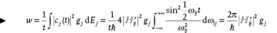c2-math-0111

where the last but one step can be made if varies slowly with energy and the last step since the integral evaluates to ½πt. This result is known as Fermi's golden rule.

In fact, the energy available is slightly uncertain due to the Heisenberg uncertainty principle. Therefore, the state i is actually one out of a group having nearly the same energy and labeled A. Similarly, j is one out of a set B with nearly the same energy. The occupation probability p_i of each of the states i may change in time. If a system in state i within a set of states A makes a transition to any state within a set of states B, the one-to-many jump rate w_BA is given by Eq. (2.111). Since we are interested in the one-to-one jump rate ν_BA from any state i in group A to every state j in group B, we make the accessibility assumption – that is, all states within a (small) energy range δE, the accessibility range, are equally accessible. It can be shown that the exact size of δE is unimportant for macroscopic systems (see Justification 5.2). Hence

(2.112)

Because , we obtain jump rate symmetry ν_ji = ν_ij. This result is used in conjunction with the master equation to show that entropy always increases.

Notes

1) The energy of the universe is constant. The entropy of the universe strives to a maximum.

2) Frivol additions are the fourth law, which states that no experimental apparatus works the first time it is set up; the fifth law states that no experiment gives quite the expected numerical result [12].

3) For notation conventions, see Section 1.4.

4) The peculiar numbering of the laws of thermodynamics resulted from the fact that the importance of the zeroth law was realized only after the first law was established. The status of the zeroth law is not without dispute [13].

5) A clear presentation of the concept of force has been given by O. Redlich [13].

6) A significant objection against the use of the concept of differential δX of the variable X has been raised by Menger [14]. Essentially, his criticism boils down to the fact that dA describes progress of the variable A with time as given by (dA/dt)dt.

7) It is clear that if dP = P_ext − P_int << P_ext, dW = P_extdV ≅ −P_intdV.

8) Using the word “heat” here means, of course, that some circularity in the argument is used, since “adiabaticity” was defined as the nonability to influence the system in the absence of forces (implying no heat transfer). This circularity can be largely avoided by more elaborate considerations in the definition of adiabatic walls. See, for example, Refs [4] and [5].

9) A reversible process can be described by a path in the (A,a) state space. The internal variables of the system, collectively indicated by ξ, control the direction and rate of the processes, externally driven by a, so that any change should actually be written as dA = (∂A/∂ξ)(∂ξ/∂a)(∂a/∂t)dt, keeping the criticism of Menger in mind. Limiting ourselves to quasi-static processes the system is at any moment in equilibrium, resulting in dA = (∂A/∂a)(∂a/∂t)dt = (∂A/∂a) da.

10) No subscripts or variables in the partial derivatives implies that the various state functions U, S, etc., are expressed in their natural parameters, that is, U = U(S,a) and ∂U/∂S = (∂U(S,a)/∂S)_a, etc.

11) A clear discussion of Legendre transforms is given by Callen [3]. See also Appendix B.

12) The designation density is used for quantities expressed per unit volume, for example, using the same symbol, the number density ρ = N/V = N_AΣ_αn_α/V. If confusion is possible, we use ρ′ for mass density.

13) The chemical equilibrium conditions can also be derived similarly as those for thermal and mechanical equilibrium.

14) We use direct instead of matrix notation, since otherwise a matrix designation for the outer product of vectors is needed. The penalty is the need of summation signs. Note that a subscript labels a particle.

15) Note that r is a vector and r is a (column matrix of a) set of elements r_i or r_i (see Section 1.4).

16) For a Hermitian operator it holds that , where the integration is over all of the domain of the functions f and g. Linearity implies , with c₁ and c₂ as constants.

17) An operator, denoted by (or by A if it is just a function), operating on any function Ψ(r) yields another function, say Ψ′(r), that is, . If the operator operating onΨ(r) yields a multiple of Ψ(r), say aΨ(r), the resulting equation is an eigenvalue equation. The function Ψ(r) is the eigenfunction, and the scalar a is the eigenvalue. Because every physical property is real, the eigenvalue must be real and this requires the operator to be Hermitian.

18) The association with brackets is obvious but the meaning of the bra <Ψ | and ket |Ψ > is much deeper, see Ref. [8].

19) Virtually the only realistic one is the hydrogen atom, at least if a nonrelativistic Hamilton operator is used. Fortunately, several model systems can be solved exactly.

20) Neglecting relativistic terms, spin interactions and the possibility of explicit time dependence.

21) In the atomic unit system the length unit is the Bohr radius, 1 a₀ = (4πε₀)ħ²/me² = 0.529 × 10⁻¹⁰ m, and the energy unit is the Rydberg, 1 Ry = me⁴/2(4πε₀ħ)² = 2.18 × 10⁻¹⁸ J = 13.61 eV. Here, ħ = h/2π with h Planck's constant, m and e the mass and the charge of an electron, respectively, and ε₀ the permittivity of the vacuum. In this system, e²/(4πε₀) = 2 and ħ²/2m = 1. Unfortunately, another convention for the energy atomic unit also exists, that is, the Hartree, 1 Ha = 2 Ry. In the Rydberg convention the kinetic energy reads −∇² and the electrostatic potential 2/r, while in the Hartree convention they read −½∇² and 1/r, respectively. Chemists seem to prefer Hartrees, and physicists Rydbergs.

References

1 Clausius, R. (1865) Pogg. Ann. Phys. Chem., 125, 353.

2 See Waldram (1985).

3 See Callen (1985).

4 See Woods (1975).

5 See Pippard (1957).

6 See Lanczos (1970).

7 See Landau and Lifshitz (1976).

8 Dirac, P.A.M. (1957) The Principles of Quantum Mechanics, 4th edn, Clarendon, Oxford.

9 See Pauling and Wilson (1935).

10 However, see Appendix VIII of Born, M. and Huang, K. (1954) Dynamical Theory of Crystal Lattices, Oxford University Press, Oxford.

11 Pilar, F.L. (1968) Elementary Quantum Chemistry, McGraw-Hill, London.

12 Kuhn, T.S. (1977) The Essential Tension, University of Chicago Press, Chicago.

13 Redlich, O. (1968) Rev. Mod. Phys., 40, 556.

14 (a) Menger, K. (1950) Am. J. Phys., 18, 89; (b) Menger, K. (1951) Am. J. Phys., 19, 476.