Liquid-State Physical Chemistry: Fundamentals, Modeling, and Applications (2013)

As indicated in Chapter 1, in liquids a natural reference state is absent because the structure is highly irregular. Therefore, in the description of liquids and solutions, we essentially will need statistical thermodynamics, which provides the link between the microscopic considerations and concepts to the macroscopic – in particular thermodynamic – aspects. In this chapter we introduce and outline statistical thermodynamics in a concise way. First, we deal with the basic formalism and apply that to noninteracting molecules. Thereafter, the effect of intermolecular interactions is introduced, leading to the virial description. While being a reasonable approach for low- and medium-density fluids, the virial approach does not work for liquids. The reasons for this are briefly discussed.

5.1. Statistical Thermodynamics

While classical or phenomenological thermodynamics provides relations between macroscopic properties, statistical thermodynamics relates the macroscopic pro­perties of a system (set of molecules) to the microscopic phenomena – that is, to molecular behavior.

5.1.1 Some Concepts

Let us try to describe a system by classical mechanics (CM). If the system is relatively small, say a single molecule or particle, one may proceed as follows. In classical mechanics the system is described by Hamilton's equations (see Section 2.2). Each system can be characterized by a set of n generalized coordinates (degrees of freedom) and the associated momenta. A state of a system thus can be depicted as a point in a 2n-dimensional (Cartesian) space whose axes are labeled by the allowed momenta and coordinates of the particles of the system. This space is called the (molecule) phase space or μ-space. Example 2.2 provides a possible choice of generalized coordinates for the water molecule. If we have a system containing many (not or weakly interacting) particles, such as molecules in a volume of gas, a collective of points describes the gas in μ-space, each point describing a molecule. Similar considerations hold in quantum mechanics (QM), which yields the energy levels and associated wave functions of individual quantum systems. However, in many cases we need the time average behavior of a macroscopic system. There are four problems to this:

· The size of the macroscopic system, which contains a large number of particles. The large number of degrees of freedom present renders a general solution (both in CM and in QM) highly unlikely to be found.

· The initial conditions of such systems are unknown so that, even if a general solution was possible in principle, a particular solution cannot be obtained.

· Even if the initial conditions were known, they have a limited accuracy. Note that, for example, Avogadro's number is “only” known with an accuracy of 10⁻⁷. Since it appears that the relevant equations are extremely sensitive to small changes in initial conditions, this rapidly leads to chaotic behavior.

· It is difficult to incorporate interaction between the molecules and the interaction with environment.

To overcome the aforementioned problems, in 1902 Gibbs made a major step and used the ensemble – a large collection of identical systems with the same Hamilton function but different initial conditions. By taking a 2nN-dimensional space, where N is the total number of particles in the system, we can make a similar representation as before. The axes are labeled with the allowed momenta and coordinates of all the particles. This enlarged space is called the (gas) phase space or Γ-space. To each system in the ensemble there corresponds a representative point in the 2nN-dimensional Γ-space. Since the system evolves in time, the representative point will describe a path as a function of time in Γ-space, and this path is called a trajectory. From general considerations of differential equations it follows that through each point in phase space (or phase point) can pass one and only one trajectory so that trajectories do not cross. The ensemble thus can be depicted as a swirl of points in Γ-space, and the macroscopic state of a system is described by the average behavior of this swirl. Since the macroscopic system considered has a large number of degrees of freedom, the density of phase points can be considered as continuous in many cases; this density is denoted by ρ(p,q), where p and q denote the collective of momenta and coordinates, respectively. Obviously, ρ(p,q) ≥ 0 and we take it normalized, that is, ∫ρ(p_,q)d p d q = 1. One can prove from the equations of motion that this density is constant if we follow along with the swirl, a general theorem called Liouville's theorem. A function F(p,q) in phase space representing a certain property is called a phase function, the Hamilton function providing an important example. The time-average of a phase function is given by

(5.1)

However, as stated before, this average cannot be calculated in general since neither the solution p = p(t) and q = q(t) nor the initial conditions p = p(0) and q = q(0) are known. To obtain nevertheless estimates of properties the phase-average

(5.2)

is introduced. The assumption, originally introduced by Boltzmann in 1887 for μ-space and known as the ergodic theorem, is now that

(5.3)

and essentially implies that each trajectory visits each infinitesimal volume element of phase space. This assumption has been proven false but can be replaced by the quasi-ergodic theorem, proved by Birkhoff in 1931 for metrically transitive systems¹⁾. It states that trajectories approach all phase points as closely as desired, given sufficient time to the system. In practice, this means that we accept the equivalence of the time- and phase-average. For details (including the conditions for which the theorem is not valid) we refer to the literature.

5.1.2 Entropy and Partition Functions

We will develop statistical thermodynamics using a quantum description, since that approach is conceptually simpler, and in a later stage make the transition to classical statistical thermodynamics. However, the terminology of classical statistical mechanics is frequently used in the literature, even when dealing with quantum systems.

The first question is how to characterize a macroscopic state in terms of molecular parameters. It might be useful to recall that a macroscopic system is considered to possess a thermodynamic or macro-state, characterized by a limited set of macroscopic parameters, such as the volume V and the temperature T. However, such a system contains many particles, for example, atoms, molecules, electrons and photons. A macroscopic system is thus also a quantum system – that is, an object that contains energy and particles and is identified by a large set of distinct quantum or micro-states of the system. Identical particles – for example, the electrons of a molecule – are objects that have access to the same subset of micro-states. From these considerations we conclude that each macro-state contains many micro-states, and describe the macroscopic state of the system by the fraction p_i of each possible quantum state i in which the macroscopic system remains. With each quantum state i an energy E_i and a number of particles N_i is associated. It should be clear that the simple label i implicates the complete description of the microstate while the distribution over microstates i describes the macroscopic system, and thus the whole hides a considerable complexity.

Further, it should be clear that the number of quantum states increases rapidly with increasing energy. For large systems, the states of the system will form a quasi-continuum that can be described by the density of states g, indicating the number of quantum states dn for a certain energy range δE, that is,

(5.4)

where δE represents the so-called accessibility range, that is, an energy range that is small as compared to E but large when compared to the Heisenberg uncertainty ΔE. For a macroscopic system g is astronomically large, is related to the temperature (see Problem 5.4), and increases extremely rapidly with the size of the system (see Example 5.1).

Example 5.1: The density of states for translation*

First, we calculate the volume G of a hypersphere with radius R and of dimension D, given by G = AR^D = A(R²)^D/2. To calculate A we consider the integral

with Γ(t) the gamma function. The volume can also be written as G = ∫ h(R²−x^Tx) dx with h(t) the Heaviside function and . So, dG/dR² = ∫δ(R²−x^Tx)dx where the Dirac function δ(t) = dh(t)/dt is used. For the functions used, see Appendix B. Therefore, the integral I also becomes

Combining yields A = 2π^D/2/DΓ(D/2) = π^D/2/Γ(½D + 1). Consider now N particles of mass m in a three-dimensional box with edges a so that the energy E can be written as where n = n_i covers the set n_1x, n_1y, … , n_Nz with n_i ∈ (±1, ±2, ±3, … ). The degeneracy of energy levels is given by the number of ways the integer n^Tn = 8ma²E/h² can be written as a sum of squares of integers. To estimate the degeneracy, consider a D-dimensional space (D = 3N) with the axes labeled n. The number of lattice points inside the hypersphere with radius squared n^Tn = 8ma²E/h², gives the number of energy levels. Equating n^Tn to R², we have

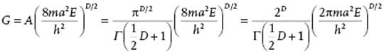
with D = 3N. The final step is to realize that we need only one “octant” of the hypersphere, so we have to divide by 2^D, and that the particles are indistinguishable, so we have to divide by N! (see Section 5.2). The final result for the volume G and density of states g(E) thus becomes, respectively,

For N = 1, using E = 3kT/2, T = 300 K, m = 10⁻²² g, and a = 10⁻² m, we obtain g ≅ 10³⁰, which is a large number. For N particles, using again T = 300 K, m = 10⁻²² g and a = 10⁻² m, but now with N = 6 × 10²³ and E = 3NkT/2, we obtain g ≅ 10^N, which is an extremely large number. Finally, the expression for g shows that it increases extremely rapidly with the number of particles in the system.

Since in thermodynamics equilibrium is reached at maximum entropy S(U,V,N), given energy U, volume V and number of particles N, it seems natural in statistical thermodynamics to start with defining the entropy. For the statistical representation of S various expressions can be given²⁾. Since the macroscopic system is characterized by the p_is, we will have S = S(p_i;U,V,N), or S(p_i) for short. Probably the most direct way to obtain S for a system having n states is to require the following properties:

· S(p_i) ≤ S(1/n). This statement implies that equi-probability for states with the same energy yield the maximum entropy and thus the equilibrium state.

· S(p_i,0) = S(p_i). This statement requires that if a state cannot be occupied it will not contribute to the entropy.

· S = S_A + S_B for noninteracting systems A and B. This condition delivers the usual additivity of entropy. For interacting systems the condition changes to , where denotes the conditional entropy of system B, that is, the entropy of system B given the entropy of system A.

These requirements have a unique solution (see Justification 5.1) apart from a multiplicative constant. This constant is chosen in such a way that the statistical entropy thus defined corresponds to the conventional thermodynamic entropy, and this constant appears to be Boltzmann's constant k. The entropy S, sometimes called Gibbs entropy, is then defined by

(5.5)

Justification 5.1: The Gibbs entropy*

To show that, given the three properties indicated above, Eq. (5.5) represents the unique solution for the entropy, we argue as follows [2]. First, as an abbreviation, we set

Using properties 1 and 2 we have

so that L(n) is a nondecreasing function of n. Now, taking m and r as positive integers, consider m mutually independent systems A₁,A₂, … ,A_m, each containing r equally likely states. So, we have S(A_k) = S(1/r, … ,1/r) = L(r) for 1 ≤ k ≤ m. Using property 3, since the systems are independent, we have

Since the combined (product) system A₁A₂ … A_m contains r^m equally likely events, we have for its entropy also L(r^m) and therefore

This relation holds for any other pair of integers m and r. As a next step, take three arbitrary integers r, s and n and a number m determined by

(5.6)

Since L(n) is monotonous we have also

(5.7)

By combining Eqs (5.6) and (5.7) we have

(5.8)

Equation (5.8) is independent of m, and since n can be arbitrarily large we obtain

which implies, since r and s are arbitrary, that L(n) = λ lnn, with λ ≥ 0 a non-negative constant as L(n) is monotonous.

So far, the special case p_i = 1/n (1 ≤ k ≤ n) is proved and now we turn to the case where p_k can be any rational number. Suppose we have p_k = g_k/g with g = Σ_kg_k where the g_k are all positive integers. Further suppose that we have a system A consisting of n states with probabilities p₁,p₂, … ,p_n. We also have a specially devised system B, dependent on A and consisting of n groups of states such that the kth group contains g_k states. If state A_k is realized in system A, then in system B all the g_k events of the kth group have the same probability 1/g_k, while all the events of the other groups have probability zero. In this case the system B reduces to a system of g_k equally probable states with conditional entropy . This implies that

We turn now to the product system AB containing A_kB_l states (1 ≤ k ≤ n, 1 ≤ l ≤ g). A state in this scheme is only possible if B_l belongs to the kth group, so that the number of possible states A_kB_l for a given k is g_k. The total number of states in system AB is then Σ_kg_k = g, and the probability of each possible state A_kB_l is p_k/g_k = 1/g. Thus, the system AB consists of g equally likely states and thus S = L(g) = λ lng. We now use property 3, S = S_A + S_B^(A), to obtain

(5.9)

Since the entropy must be continuous, Eq. (5.9) is not only valid for the rational numbers p₁,p₂, … ,p_n but for any value of its arguments. Note that, although we used a specially devised system B, the result is independent of system B. Finally, the constant λ can be identified with Boltzmann's constant k by calculating the pressure for a perfect gas, Eq. (5.33). This leads to λ = k, which we use from now on.

A short route to obtain the relevant thermodynamic expressions runs as follows. We assume an open system³⁾, that is, a system of volume V to be in contact with a thermal bath characterized by the temperature T, and a particle bath characterized by the chemical potential μ⁴⁾. Alternatively, we may assume that the system is in contact with many other, similar systems. For such a system we may assume that we are always near equilibrium. The probabilities of the system ought to be normalized⁵⁾, that is,

(5.10)

In addition, we require that the average energy of the system⁶⁾ is constant, that is,

(5.11)

and that the average number of particles ⟨N⟩ of the system is constant, that is,

(5.12)

We use the expression for the entropy considered before, S = −kΣ_i p_ilnp_i, and for this expression we seek, conform thermodynamics, the maximum given the above-mentioned constraints. This maximum can be obtained by using the Lagrange method of undetermined multipliers (see Appendix B). We take these multipliers as −kα, −kβ, and −kγ. The maximum is now obtained from

(5.13)

and after some calculation this expression leads to the solution

The normalization condition, Eq. (5.10), yields

so that we may define

For the probabilities we thus obtain

The function Ξ is the macro-canonical or grand canonical partition function, often just called the grand partition function. We find for the entropy, meanwhile using the normalization condition ,

We compare this expression with the thermodynamic expression for the entropy

as solved from U = TS − PV + μN (see Section 2.1) with T, μ, and P as before, and U the internal energy, N the number of particles, and V the volume. If we identify the average microscopic energy with the internal energy U, the average number of particles ⟨N⟩ with the macroscopic number N, we obtain

(5.14)

so that we finally have the solution

(5.15)

Since we are only using the values of p_i corresponding to the maximum entropy, in the sequel we omit the asterisk and just write p_i. For future reference, we also write the expressions⁷⁾ for p_i and Ξ as

(5.16)

(5.17)

where λ is the absolute activity (see Section 2.1). The grand partition function is directly related to the grand potential Ω, since we have −PV = Ω and thus Ω = −kT ln Ξ. The thermodynamic properties can be calculated in the usual thermodynamic way by realizing that the natural variables for Ξ are T, V and μ, that is, Ω = Ω(T,V,μ). Hence, we have S = −∂Ω/∂T, P = −∂Ω/∂V, and N = −∂Ω/∂μ.

If the number of particles is fixed at, say N, we have a closed system, the constraint characterized by γ is removed, and one can take γ = 0. Therefore,

(5.18)

Here, Z_N denotes the canonical partition function for N particles, often labeled as just Z and addressed as the partition function. For the entropy we have in this case

which, upon comparison with

results again in β = 1/kT, as expected, and F = − kT ln Z. From the Helmholtz energy F we obtain the internal energy U, the entropy S, pressure P, and chemical potential μ

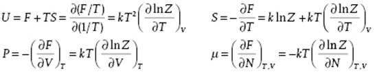
We note that using Z_N we can write Ξ = Σ_Nλ^NZ_N, where the original index i has been replaced by the pair (N,j) with j the index used in Z_N.

Finally, if also the energy is fixed, we have an isolated system, the constraint characterized by β is also removed and one can take β = 0 as well. In this case the probabilities p_i reduces to the micro-canonical distribution

where W = Σ_i(1) is the number of accessible states for the macroscopic system at fixed energy E⁸⁾. In this case, the entropy S(p_i) = −k Σ_i p_i lnp_i becomes the Boltzmann relation

(5.19)

Writing this expression as −TS = −kT ln W renders the expressions for the relation between the potentials (Ω = −PV = U − TS − μN, F = U − TS, −TS) and the partition functions (Ξ, Z, W) all similar. Once having calculated the p_is, the mean or average value for any property X of the system can be calculated using

(5.20)

where X_i denotes the value in microstate i. This expression is valid for all three distributions discussed. Note that adopting this view we can write for the entropy S = −k Σ_ip_ilnp_i = −k<lnp>.

To show that the entropy just defined (for all situations) can be identified as the thermodynamic entropy (defined for equilibrium situations only), we calculate dS for a closed system using lnp_i = −E_i/kT − lnZ and obtain

(5.21)

Here, we have used the definition of the Boltzmann distribution and twice the fact that ∑_i dp_i = 0. Hence, for reversible heat flow we have δQ = T dS = Σ_i E_i dp_i. The total energy of the system of interest and its differential d. From thermodynamics we know that the internal energy U is given by the first law of thermodynamics dU = δW + δQ, where δW and δQ denote the increment in work and heat, respectively. If we again identify U with , we can associate Σ_i p_idE_i with δW since Σ_i E_idp_i corresponds to TdS = δQ. Finally, from Eq. (5.21) one easily can show that ∂S/∂U = 1/T (see Problem 5.1).

One property not discussed so far is that, for the thermodynamic entropy S, we have dS ≥ 0 for an isolated system. One can show that for the statistical entropy we also have dS ≥ 0 always (see Justification 5.2). Finally, one might wonder what the partition function represents. In fact, it just provides the average number of states that is thermally accessible for the system. This is particularly clear for the micro-canonical ensemble (S = k lnW).

Justification 5.2: dS ≥ 0 always*

One property of the thermodynamic entropy is that for arbitrary processes it will increase unless the process is reversible. To prove that our statistical entropy behaves similarly, we first have to make the meaning of micro-states somewhat more precise. In fact, for any macroscopic system it is impossible to obtain the exact eigenstates of the system. Moreover, even if we would know them at a certain moment, soon afterwards, because of the interaction between the particles in the system, they would be unknown. For example, for an ideal gas the eigenstates are the described by the momentum eigenfunctions of structureless point particles. During equilibration the particles collide and exchange momentum. The uncertainty in energy E thus becomes ΔE ≥ ħ/2Δt, where Δt is the mean time between collisions. As indicated in footnote 7, experimentally we are limited to δEwith δE >> ΔE. Hence, generally we have groups of approximate eigenstates associated with a small energy range, the accessibility range δE, small as compared to E but large as compared to the Heisenberg uncertainty ΔE and in which the density of states is essentially constant. The probabilities p_i therefore refer to these approximate states and, when δE is small enough, can be considered as constant within the accessibility range. It then makes no difference whether we consider transitions from exact state i to exact state j as restricted by ΔE or transitions from one approximate state (group) i to another state (group) j as restricted by δE: in either case, the value of dp_i/dt will be the same. This assumption is equivalent to the ergodic assumption as it also realizes mixing of all states. Sometimes it is referred to as the accessibility or equal a priori probabilityassumption.

To discuss equilibration we need the jump rate ν_ij from state j to state i. For the rate at which a state i with probability p_i is changing, we have two contributions. First, we have the contribution from state i to any state j, given by Σ_jν_ji p_i and, second, the contribution from any state j to state i, given by Σ_jν_ij p_j. Quantum mechanics tells us that ν_ij = ν_ji, that is, the principle of jump rate symmetry (see Section 2.4), and therefore the total rate becomes dp_i/dt = Σ_jν_ij(p_j − p_i), referred to as the master equation.

We now consider the entropy differential dS/dt = −k Σ_ilnp_i (dp_i/dt). For an isolated system we have for the effect of jumps between two particular states i and j a contribution to dp_i/dt reading ν_ij(p_j − p_i) as well as a contribution ν_ij(p_i − p_j) to dp_j/dt. The total rate is thus, taking in to account all jumps, dS/dt = kΣ_i,jν_ij(p_j − p_i)(lnp_j − lnp_i). Since the terms in brackets have the same sign, dS/dt cannot be negative. Moreover, if p_i = p_j, dS/dt = 0, and so we conclude that always dS ≥ 0. We refer to the literature for a further discussion of the foundations of statistical thermodynamics [3].

5.1.3 Fluctuations*

We note that the difference between the results from the grand partition function Ξ and the partition function Z is usually small for macroscopic systems, that is, fluctuations in the number of molecules and therefore energy, are gen­erally not terribly important. This can be seen as follows. The grand partition function is

(5.22)

where Z_N is the canonical partition function for N particles, so that the probability to have N particles in the system is

(5.23)

Hence, it follows that

(5.24)

Noting that since ⟨N⟩ = ∂lnΞ /∂lnλ, differentiation of ⟨N⟩ with respect to μ yields

where the variance σ_X² ≡ ⟨X²⟩ − ⟨X⟩² is used. We also have

Since the derivative (∂N/∂P)_V,T is at constant V, we have (∂N/∂P)_V,T = V[∂(N/V)/∂P]_V,T = V[∂(N/V)/∂P]_N,T = NV[∂(1/V)/∂P]_N,T = Nκ_T, where the second step can be made because N/V is an intensive quantity. Therefore, we have . Hence, the relative fluctuation in number of molecules in the system is given by

and therefore for large N is negligible. The fluctuation in energy for an open system can be derived similarly, although the process is somewhat more complex, and we quote (leaving the derivation for Problem 5.6)

Problem 5.1

Show, using Eq. (5.21), that ∂S/∂U = 1/T.

Problem 5.2

Verify from the thermodynamic expression for dU and the statistical expression for dS that δW in the grand canonical ensemble is given by

Problem 5.3: The two-state model

A very simple model in statistical mechanics is the two-state model with (obviously) two states, state 1 with energy 0 and state 2 with energy ε.

a) Give the expression for the partition function Z.

b) For temperature T = ε/k, where k is Boltzmann's constant, calculate the occupation probabilities of state 1, p₁, and of state 2, p₂.

c) Calculate the internal energy U.

d) Calculate the heat capacity C_V and sketch the behavior of C_V(T).

Problem 5.4: Temperature and the density-of-states

Show that the temperature T is related to the density of states g(E) for a system with energy E_s via .

Problem 5.5

Show in detail for macro-systems, although we have S = g(E)δE, that S is essentially independent of δE. Consider to that purpose the value of δE based on the quantum uncertainty relations and a typical experimental uncertainty.

Problem 5.6*

Derive for a closed system in a way similar as the relation (σ_N/<N>)² = kTκ_T/V is derived for the open system. For an open system, show that .