Liquid-State Physical Chemistry: Fundamentals, Modeling, and Applications (2013)

5.6. Real Gases

Statistical thermodynamics provides a useful description of (nearly) perfect gases, that is, low density gases, proof being that the values of the standard entropy S_m° can be calculated in precise agreement with experimental data¹⁴⁾. Example 10.2 illustrates this. We need, of course, also a description of nonperfect gases, and to that purpose we need to introduce the interaction potential in the partition function.

5.6.1 Single Particle

Let us recapitulate the results for the partition function z of a single particle with mass m, momentum p₁ and (Cartesian) coordinate r₁ enclosed in a box with edge l (and volume V = l³). The energy E is only kinetic and given by the Hamilton function so that

The partition function z is given by

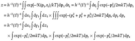
Evaluating this expression results, as before, in the partition function

(5.51)

with Λ = (h²/2πmkT)^1/2 the thermal wavelength.

5.6.2 Interacting Particles

Let us now evaluate the partition function for two interacting particles, characterized by the set of variables (p,r) = (p₁,r₁,p₂,r₂) and their potential energy of interaction ϕ(r₁,r₂). In this case, the energy is given by

Actually, the potential energy ϕ can be written as ϕ(r₁,r₂) = ϕ (r) with r = |r₂ − r₁| if we assume that ϕ is spherically symmetrical and thus only depends on the distance r between the two particles. Thus, we obtain for the partition function

(5.52)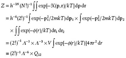

The factor Q₁₂ is usually addressed as the (two particle) configuration integral.

This result can be easily generalized to N particles, characterized by (p,r) = (p₁, r₁, p₂, r₂, … , p_N, r_N) and Φ(r) = Φ(r₁,r₂, … , r_N). The total energy is

Assuming again spherically symmetrical interactions between the particles we have

where r_ij denotes the distance between particle i and particle j. The partition function becomes

(5.53)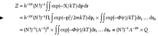

with Q the configuration integral. Our remaining task is thus to evaluate this many-dimensional integral.

5.6.3 The Virial Expansion: Canonical Method

The method we use in this paragraph to evaluate Q is denoted as the virial expansion. There are several ways to do this and we use the simplest possible. The first thing we assume is that we can write the potential Φ in the expression for

(5.54)

as Φ (r) = Σ_i<jϕ (r_ij) = ½Σ_i,jϕ (r_ij). This allows us to rearrange the exponential of the sum as the product of exponentials since exp(−Σ_ia_i) = Π_i exp(−a_i). Applying this operation to the configuration integral, meanwhile using exp(ab) = (exp a)^b, we have

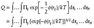
The trick is now to introduce the Mayer function f_ij = exp[−ϕ(r_ij)/kT] − 1 so that

(5.55)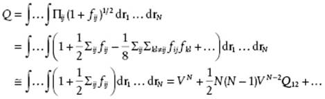

(5.56)

where in the last line particle 1 is taken as the origin so that the integration over particle 1 yields the volume and the remaining integration is only over the distance r. The final result, assuming N(N − 1)b₂/V << 1, is

(5.57)

In the canonical ensemble the pressure P can be calculated using P = −∂F/∂V = kT ∂lnZ/∂V = kT ∂lnQ/∂V and reads PV/nRT = 1 + B₂/V + … with B₂ = −b₂ (Problem 5.27) or βP = ρ + B₂ρ² + … with ρ = N/V and β = 1/kT. However, in general the expression for ϕ is complex so that analytical evaluation of b₂ is almost never possible and we have to resort to numerical integration.

Example 5.3: The hard-sphere second virial coefficient

A simple potential energy expression for which an analytical evaluation of b₂ is possible is the hard-sphere model,

We split the integration for b₂ from 0 to ∞ in 0 to σ and from σ to ∞. The first integral reads , while the second integral results in . The total result is thus B₂ = −b₂ = 2πσ³/3.

From Example 5.3 we note that b₂ < 0, and this appears generally to be the case (see Chapter 4). For convenience often the quantity b ≡ B₂ = −b₂ = 2πσ³/3 is defined and used as a reference value in more extended calculations, and we do so likewise. Guggenheim refers to gases which can be described reasonably well by using only the second virial coefficient B₂ as “slightly imperfect gases”.

The excess Helmholtz energy F^E = F − F^idg can be written as with the ideal gas Helmholtz energy βF^idg = N ln(ρ/ρ°) where ρ° is a reference density. The coefficients are related to the pressure virial coefficients, and can be shown by integration to be

(5.58)

5.6.4 The Virial Expansion: Grand Canonical Method*

There is a problem with the derivation given in the previous section. It is assumed that the correction terms are small. For the first correction term with respect to the perfect gas this implies that (N(N − 1)/V)b << 1. Assuming b to be of the order of the molecular volume, one can easily calculate that this is not the case. Another approach is thus required and the shortest is via the grand canonical partition function.

Recall that the grand canonical partition function reads

(5.59)

and Z_N is the canonical partition function for N particles, which thus includes all energies belonging to the state containing N particles. For consistency, Z₀ is defined as Z₀ = 1, while Z₁ represents the situation containing one particle and is thus Z₁ = Vz_int/Λ³, where z_int represents the internal contributions. We will neglect the latter and thus use Z₁ = V/Λ³ = Q₁/Λ³, since for a single particle the configurational partition function equals the volume. This implies that the partition function becomes

(5.60)

where Q_N is the configurational partition function for N particles and that Ξ reads

(5.61)

Let us now assume that we may expand the pressure in a power series in ξ, that is,

(5.62)

so that the grand partition function, using exp(x) = 1 + x + x²/2 + … , becomes

(5.63)

(5.64)

(5.65)

Comparing terms with , Eq. (5.61), yields

(5.66)

(5.67)

(5.68)

From the expression for the number of particles

(5.69)

we obtain the number density

(5.70)

Inverting this series we write

(5.71)

and substitute this expression in the one for ρ, Eq. (5.70), to obtain

(5.72)

so that the coefficients a_i become

(5.73)

(5.74)

(5.75)

Now these coefficients are used in the series for ξ, Eq. (5.71), and we obtain

(5.76)

The final step is made by substituting this expression in the expression for βP, Eq. (5.62), and the result reads

(5.77)

(5.78)

(5.79)

Comparing this result with the virial expansion βP = ρ + B₂ρ² + B₃ρ³ + ···, we obtain

(5.80)

For B₂ the final result is thus

(5.81)

(5.82)

The final result for B₂ using the grand canonical partition function thus agrees with the result from the canonical partition function. However, in the former case B₂ is the coefficient of a small term while in the latter case it is the coefficient of a large term, rendering the expansion rather doubtful. It also shows that the second virial coefficient is strictly dependent only on two-body interactions. This applies also to the higher-order terms: the nth order virial coefficient is only dependent on the n-body interactions (and the lower-order ones). The virial expansion has also been derived without making the pair potential assumption [11] as well as with an entirely different method [12].

5.6.5 Critique and Some Further Remarks

A systematic extension of the virial expansion can be realized, although this is usually performed via a graphical technique known as the cluster expansion (see Ref. [13]). This extension is required when we wish to apply the virial expansion to higher densities, such as those of liquids. As mentioned in Chapter 1 (and further discussed in Chapter 6), the coordination number of a reference molecule in a liquid is generally about 10. Recalling that the nth virial coefficient deals with n-body interactions, a description of liquids in terms of the virial equation thus requires virial coefficients at least up to order 10. The calculation of high-order virial coefficients is rather complex, even for a simple potential like the hard-sphere potential. While the third and fourth virial coefficients for the hard-sphere potential can be calculated analytically, the values for the higher-order coefficients are obtained from simulations. The virial coefficients for the hard-sphere gas up to B₁₀ is shown in Table 5.2. For more realistic potentials, however, usually only the second or, maybe the third or fourth coefficient is available. Hence, for liquids we encounter problems in view of the high coordination numbers.

Table 5.2 Virial coefficients of the hard-sphere fluid in terms of B₂ = b = 2πσ³/3.^a)

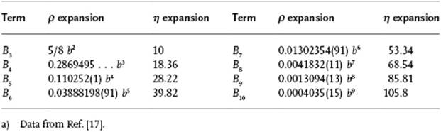
From the data in Table 5.2 it is be clear that the convergence of the virial expansion is not rapid. This is even made clearer if we introduce the close-packed volume, that is, the volume per molecule for a FCC lattice given by of spheres with diameter σ, as the reference volume. Introducing the packing fraction (or reduced density) η = N(4π/3)(σ/2)³/V = ρπσ³/6 = ρb/4 = 2^1/2πV₀/6V, the virial expansion can also be expressed in η instead of ρ. Note that for the packing fraction we have 0 ≤ η ≤ 2^1/2π/6 ≅ 0.7405.

(5.83)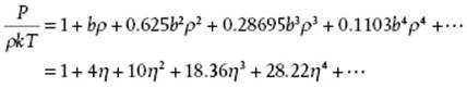

For hard-spheres, P/ρkT ≥ 1 and continuously increases with ρ. A comparison of the virial results including B₁₀ with those of computer simulations [14] shows that they begin to deviate at ρσ³ ≅ 0.5 or η ≅ 0.26. However, a 5,4 Padé approximant¹⁵⁾ to the first six hard-sphere virial coefficients reading

(5.84)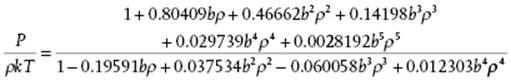

provides an excellent agreement with molecular simulation results, that is, a deviation less than 0.3% over the complete range [14].

A few problems exist when the virial expansion is applied to liquids; already mentioned are the availability and complexity of virial coefficient calculations and the slow convergence. However, real convergence problems exist with the virial expansion at certain densities and temperatures, as it converges only in some nonzero region, although in that region convergence occurs for a wide class of potentials. Essentially, and if the expansion diverges. Perhaps more important, the virial expansion does not predict a transition from gas to liquid at high density. Monte Carlo computer simulations [15] have shown that for the hard-sphere system a freezing transition occurs at η = 0.494 ± 0.002 (V/V₀ = 1.50) from a fluid, disordered phase to a solid, ordered closed-packed phase with η = 0.545 ± 0.002 (V/V₀ = 1.36). The melting temperature and pressure are related by P_mel = (8.27 ± 0.13) ρ₀kT_mel, where ρ₀represents the number density for the closed packed phase. The virial expansion fails to reveal this. Note that η = 0.50−0.55 is much lower than η_RCP = 0.64 or η_CP = 0.74. Hence, the regular solid phase is favored thermodynamically at a much lower density than at which the transition becomes necessary for geometric reasons. For the phase transition, several thermodynamic functions are nonanalytical which cannot be described by a finite order expansion. In the past, attempts have been made to connect the radius of convergence to condensation, but nowadays it is felt that there is no such relationship.

In summary, although the virial approach is useful for gases at intermediate density, for liquids other approaches are required. These approaches include integral equation models including thermodynamic perturbation theory, physical models and simulations. These will be discussed in the next chapters.

Problem 5.26: The square-well potential

Show that for the square-well potential as given by

(5.85)

where σ is the hard-sphere diameter and ε and Rσ are the depth and range of the square-well, respectively, that the (second) virial coefficient B₂ is given by

(5.86)

Discuss the role of the attractive part in ϕ_SW. Show that Eq. (5.86) increases continuously with T without showing a maximum (as experimentally observed) and discuss the reason why. Calculate the Boyle temperature T_B where B₂(T_B) = 0.

Problem 5.27

Show, assuming N²b₂/V << 1, that

and thus that the second virial coefficient B₂(T) = −b₂.

Problem 5.28

Show that at STP the term N²b₂/V ≈ 1.

Problem 5.29

Consider the model potential u(r) = ∞ for r < σ and u(r) = −Ar⁻ⁿ for r ≥ σ. Show that B₂ is only finite if n > 3. Use the expansion for the exponential.

Problem 5.30

Prove Eq. (5.58).

Problem 5.31

The dissociation of dimers (d) to molecules (m) can be described by x_d → 2x_m, where x denotes the mole fraction and the (mole fraction) equilibrium constant . Assume that initially N dimers are present, each with bonding energy −ε with respect to molecules, and neglect the vibration and rotation of the dimers. Show that:

a) the equilibrium constant K = 4 exp(−βε)/[2 + exp(βε)], and

b) x_d = 0.576 and x_m = 0.424 at T = ε/k.

Problem 5.32*

Evaluate using a symbolic math program, such as Maple, the second virial coefficient for the Lennard-Jones potential, and show that the result describes the experimental behavior, including the presence of a maximum, quite well.

Notes

1) A mechanical system is metrically transitive if the energy surface cannot be divided into two finite regions such that orbits starting from points in one region always remain in that region. See Ref. [1].

2) Formally, the statistical representation of the thermodynamic S should be denoted by another symbol, for example, ⟨S⟩. However, we identify right away ⟨S⟩ with S.

3) For simplicity of notation, we assume only one type of particle.

4) This implies that the conjugate variables (pressure P, energy U, and number of particles N) fluctuate.

5) Luckily, the probability of each system being in state i can also be interpreted in classical terms as the fraction of systems in the ensemble in state i. In that case, i refers, of course, to a volume in Γ-space of size h^nN, labeling a particular set (p,q).

6) We write since E represents the numerical value of the energy, while the Hamilton operator represents the energy expression (see Chapter 2).

7) Even though β is identified as 1/kT, for convenience the symbol β is still used frequently.

8) The uncertainty relations tell us that the energy E has an uncertainty ΔE. Moreover, exactly defined energies are not realizable experimentally and cover a range δE. Typically, it holds that δE >> ΔE. Hence, we have actually to write W = g(E)δE with g(E) = dn/dE the density of states and δE the accessibility range for the energy E in which we can take g(E) as constant. However, the value of the logarithm of δE is usually completely negligible as compared to ln g(E) and is therefore omitted. By the way, W is sometimes denoted as the “thermodynamic probability”. It will be clear that the use of the word “probability” is completely unjustified here.

9) This correction is overcorrecting the situation though, because in the double sum, as indicated in Eq. (5.30), the contribution ij (i≠j) is counted twice because ji represents the same physical configuration while double counting is not done for the contribution ii. This shows right away that the correction is only valid for noncondensed systems.

10) The Stirling approximation for factorials reads ln x! = x ln x − x + ½ ln(2πx) + . … This approximation is excellent even for x = 3, the difference with the exact value being about 2%. Often, the term ½ ln(2πx) is neglected. Although the latter approximation is considerably less accurate, for x = 50 it deviates only about 2% from the exact value. Since typically much larger numbers are used, the approximation ln x! = x ln x − x, or alternatively x! = (x/e)^x, is usually quite sufficient.

11) The symbolism for Z_N and Q_N is not uniformly used. In some cases the factor 1/N! is included in Q_N while in other cases the reverse designation for Z_N and Q_N is used.

12) The energy is often characterized by the frequency ν = ε/h in s⁻¹ (with B = h/8π²I) or by the wave number ϖ = ε/hc in cm⁻¹ (associated with B = h/8π²Ic).

13) Any N-atom molecule in principle has 3N − 6 internal degrees of freedom. For linear molecules this number reduces to 3N − 5 because rotation around the length axis, although possible in principle, will require extremely high energy in view of the small moment of inertia around that axis.

14) These calculations are essentially based on translation, harmonic vibration and rigid rotation as well as on the third law, that is, the residual entropy S_res = 0. For molecules such as CO with only a small dipole moment, (almost) random ordering in the lattice occurs, resulting in W = 2^N possible configurations and thus to an entropy contribution S_res = k ln W = 5.8 J K⁻¹mol⁻¹, in essential agreement with the experimental residual entropy for CO, determined as 4.5 J K⁻¹mol⁻¹.

15) In numerical analysis it is well known that a truncated power series of a function is an unsatisfactory way of approximation. A more sophisticated method is the use of Padé approximants [18] which represents the function by a ratio of polynomials. The coefficients are found by expanding the ratio, and to require they represent the first k Taylor coefficients correctly. For example, f(x) ≅ c₀ + c₁x + … c_kx^k is approximated by the n,m approximant f(x) ≅ (a₀ + a₁x + … a_{n − 1}x^{n − 1})/(1 + b₁x + … b_{m − 1}x^{m − 1}). Obviously, n + m − 1 should equal k + 1. A matrix recipe is given by Ree and Hoover [19].

References

1 Khinchin, A.I. (1949) Mathematical Foundations of Statistical Mechanics, Dover, New York.

2 Khinchin, A.I. (1957) Mathematical Foundations of Information Theory, Dover, New York. See also Landsberg (1978).

3 (a) Tolman, R.C. (1938) The Principles of Statistical Mechanics, Oxford University Press, Oxford (see also Dover Publishers reprint, 1979); (b) Waldram, J.R. (1985) The Theory of Thermodynamics, Cambridge University Press, Cambridge; (c) van Kampen, N.G. (1993) Physica, A194, 542.

4 (a) Kirkwood, J.G. (1933) Phys. Rev., 44, 31 and (1934) 45, 116; (b) Wigner, E.P. (1932) Phys. Rev., 40, 749; (c) Green, H.S. (1951) J. Chem. Phys., 19, 955.

5 (a) A detailed discussion is given by Hill, T.L. (1956) Statistical Mechanics, McGraw-Hill, New York (see also Dover Publishers reprint, 1987); (b) Landau, L.D. and Lifschitz, E.M. (1980) Statistical Physics, vol. 1, 3rd edn, Addison-Wesley, Reading, MA.

6 See Schrödinger (1952).

7 Hill, T.L. (1956) Statistical Mechanics, McGraw-Hill, London (see also Dover, 1987).

8 Knox, J.H. (1978) Molecular Thermodynamics, Wiley, Interscience.

9 See McQuarrie (1973).

10 See Lucas (2007).

11 Ono, S. (1951) J. Chem. Phys., 19, 504.

12 Yang, C.N. and Lee, T.D. (1952) Phys. Rev., 87, 404 and 410.

13 (a) Friedman, H.L. (1985) A Course in Statistical Mechanics, Prentice-Hall, Englewood Cliffs, NJ; (b) Hansen, J.-P. and McDonald, I.R. (2006) Theory of Simple Liquids, 3rd edn, Academic Press, London.

14 Bannerman, M.N., Lue, L., and Woodcock, L.V. (2010) J. Chem. Phys., 132, 084507.

15 Hoover, W.G. and Ree, F.H. (1968) J. Chem. Phys., 49, 3609.

16 McQuarrie, D.A. and Simon, J.D. (1999) Molecular Thermodynamics, University Science Books, Sausalito, CA.

17 Clisby, N. and McCoy, B.M. (2006) J. Stat. Phys., 122, 15.

18 Ralston, A. (1965) Introduction to Numerical Analysis, McGraw-Hill, New York.

19 Ree, F.H. and Hoover, W.G. (1964) J. Chem. Phys., 40, 939.

Further Reading

Chandler, D. (1987) Introduction to Modern Statistical Mechanics, Oxford University Press, Oxford.

Fowler, R.H. and Guggenheim, E.A. (1939) Statistical Thermodynamics, Cambridge University Press, London.

Landsberg, P.T. (1978) Thermodynamics and Statistical Mechanics, Oxford University Press, Oxford, UK (see also Dover, 1990).

Lucas, K. (2007) Molecular Models of Fluids, Cambridge University Press, Cambridge.

McQuarrie, D.A. (1973) Statistical Mechanics, Harper and Row, New York.

Schrödinger, E. (1952) Statistical Thermodynamics, 2nd edn, Cambridge University Press, Cambridge (see also Dover Publishers reprint, 1989).

Widom, B. (2002) Statistical Mechanics, A Concise Introduction for Chemists, Cambridge University Press, Cambridge.