Liquid-State Physical Chemistry: Fundamentals, Modeling, and Applications (2013)

In Chapter 5, an outline was provided of statistical thermodynamics and its application to noninteracting and interacting molecules in gases. Essentially, the approach did not work for liquids because the reference state (the perfect gas) is too far away from the liquid structure. Here, we take the opposite view and start from solids, and therefore we review first the structure of solids rather briefly. Thereafter, a general way to deal with the complex arrangements of atoms – that is, the use of the pair correlation function – is described and applied to explain the meaning of structure for a liquid. Together with intermolecular potentials, this function leads to expressions for the energy and pressure in liquids – that is, to the equations of state of liquids.

6.1. The Structure of Solids

Before embarking on the structure of liquids, we briefly review the structure of solids [1]. Recall that a crystal can be considered as a regular stacking of unit cells described by three (not necessarily orthogonal) noncoplanar basis vectors. In ideal solids, each crystallographic unit cell contains the same amount of matter in the same configuration. To create a crystal structure, it is necessary to arrange points in space in such a way that each of these points has an identical neighborhood. Stacking of the unit cells in this way can be achieved in only 14 ways in 7 crystal systems, resulting in the so-called Bravais lattices. If these points are actually occupied by molecules¹⁾ and no other molecules are present in the cell, we have a primitive lattice whereas, in the case of more molecules occupying the unit cell, we speak of a lattice with a basis.

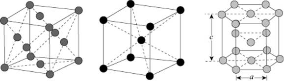
The crystal structure of many compounds is based on a limited number of simple stackings. These are the simple cubic (SC), face-centered cubic (FCC), body-centered cubic (BCC), and hexagonal close-packed (HCP) structures (Figure 6.1). While the relative theoretical density ρ_the of the SC and BCC lattice is 0.524 and 0.680, respectively, for the FCC and HCP lattice ρ_the = 0.741, so that a considerable difference in density exists. In a crystalline solid, essentially a limited number of type interstitial holes with a fixed fraction are present; for example, in the FCC lattice only tetrahedral holes are present whilst for the BCC only octahedral holes exist.

Figure 6.1 The FCC, BCC, and HCP structures (left to right).

In crystalline solids defects occur and it is possible to distinguish between zero- (0-D), one- (1-D), two- (2-D), and three- (3-D) dimensional defects. Whilst for a 0-D defect (i.e., vacancies or interstitials) only a single molecule deviates from the ideal crystallographic order, for 1-D, 2-D and 3-D defects a (connected) line, plane, or volume of molecules deviates from the ideal order [1]. Although by introducing defects into solids the order is disturbed, the structure remains overwhelmingly regular. For example, near the melting point, though they are thermodynamically required, in a metal typically only about 1‰ of vacancies are present. Although the activation energy for defects in many substances is much lower than for metals, to describe a structure similar to amorphous materials requires so many defects that the use of individual defects is no longer warranted.

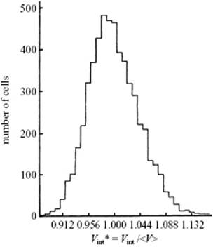
A useful description of amorphous materials, represented by a random dense packed structure of single-sized spheres as first presented by Bernal, is given in terms of polyhedral shapes of the interstitial holes. Five basic types of hole could be discerned (Figure 6.2), sometimes referred to as the canonical holes. The actual holes are somewhat distorted, but a random packing contains a certain fraction of each type [2] (Table 6.1); their frequency represents the frozen structure. The average number of nearest neighbors for each sphere is about nine, compared to 12 for the FCC lattice. The relative density for a structure of random close-packed spheres is about 0.637, compared with ρ_FCC = 0.741 and ρ_BCC = 0.680. On average, the volume per molecule is thus about 15% larger than the volume per molecule for a FCC crystal, corresponding to a lower average coordination number. The excess volume is referred to as the free volume. This already hints at another means of characterizing a glassy structure, namely the distribution of the volume per molecule. In an ideal crystal the volume per molecule is the same for every molecule. In an amorphous material there are molecules with a surrounding for which the volume per molecule is less than for a random close-packed structure, while others have a larger volume and there is a considerable width for this distribution [3] (Figure 6.3).

Figure 6.2 The five canonical holes of Bernal.

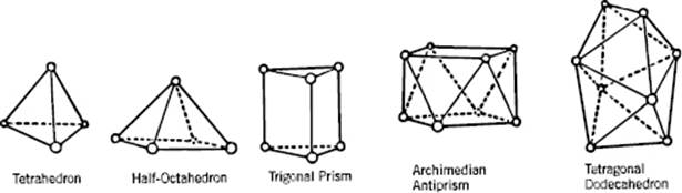
Table 6.1 Relative frequency of canonical holes.

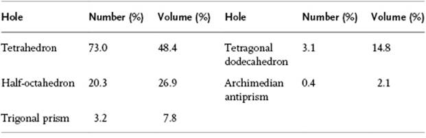
Figure 6.3 The volume per sphere distribution for a random packing of spheres with the maximum at V_int* = V_int /⟨V⟩ = 0. 984 with ⟨V⟩ = 0.637 the random close-packed relative density.

Although the picture sketched so far is static, molecules in any structure will vibrate around their equilibrium positions. Despite the molecular motions being correlated, in the simplest approach these correlations are neglected. This model was first introduced by Einstein, and accordingly denoted as the Einstein model. In this model it is supposed that all molecules vibrate independently around their equilibrium positions with the same circular frequency ω, denoted as the Einstein frequency. As these vibrations are treated quantum-mechanically, the energy levels of a quantum oscillator are needed to calculate its average behavior (see Chapter 2). Although this description is clearly flawed, it describes the thermal behavior of solids reasonably well to first order, and is therefore often used.

Problem 6.1

Using Figure 6.3, estimate the density of the glass relative to that of the crystal. Also estimate the local density variations that can be expected.