The Potential of Mean Force - Describing Liquids: Structure and Energetics - Liquid-State Physical Chemistry: Fundamentals, Modeling, and Applications (2013)

Liquid-State Physical Chemistry: Fundamentals, Modeling, and Applications (2013)

6. Describing Liquids: Structure and Energetics

6.6. The Potential of Mean Force

It is useful to define a quantity W^(s)(r₁, … , r_s) by

(6.51)

where the definition of the correlation function g^(s)(r₁, … , r_s) is given by

(6.52)

Taking logarithms on both sides, and then taking the gradient with respect to one of the particles, say i, one obtains

(6.53) 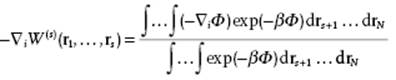c6-math-0053

Since −∇_iΦ represents the force on molecule i for a fixed configuration of r₁, … , r_s, the right-hand side is the mean force averaged over the configurations of all molecules s + 1, … , N not in the fixed set 1, … , s. Therefore,

(6.54)

Since a force F_j on particle j is always calculated from the corresponding potential Ψ according to F_j = −∂Ψ/∂r_j, the quantity W^(s)(r₁, … , r_s) can be interpreted as potential of mean force (fixating s particles).

In particular, for s = 2 we have W(r₁,r₂) ≡ W⁽²⁾(r₁,r₂), representing the potential of mean force between one particle held at position r₁ and another held at position r₂. The pair correlation function g(r₁,r₂) and the pair potential of mean force W(r₁,r₂) are thus related by

(6.55)

for isotropic systems. For r (= |r₂ − r₁|) → ∞, W(r) → 0 and g → 1. From W(r) = −kT ln g(r), we see that, providing that βW(r) << 1, g(r) permits the expansion

(6.56)

For low density ρ, W(r) → ϕ(r) because the two molecules considered are no longer affected by the other molecules. Hence, at low density g(r) reduces to

(6.57)

and there is a unique correspondence between ϕ(r) and g(r). At higher density one writes, using the background correlation function y(r),³⁾

(6.58)

Since dexp(−βϕ)/dr = −β exp(−βϕ)dϕ/dr, substituting Eq. (6.58) in the pressure Eq. (6.39) leads to the expression

(6.59)

To obtain P as a function of ρ, we need the expansion for y(r) in ρ reading (and indicating but not using second-order terms)

(6.60)

so that g(r) becomes g(r) = exp[−βϕ(r)]y(r) ≡ exp[−βϕ(r)](1 + A₂₁ρ + A₂₂ρ² + …). In the same spirit, we write g⁽³⁾(r) = exp[−β(ϕ₁₂ + ϕ₁₂ + ϕ₁₂)](1 + A₃₁ρ + A₃₂ρ² + …). Substituting these expansions in the Yvon–Born–Green (YBG) equation (Eq. [7.5]),

(6.61)

we obtain for both sides of the YBG equation a polynomial in the density ρ. The next step is to equate equal order terms in ρ, and for the first-order terms in ρ this leads to

(6.62)

Integration yields

(6.63)

where C is the integration constant. Since for r₁₂ → ∞, g(r) → 1, we obtain from g(r) = exp(−βϕ)(1 + A₂₁ρ + …) as the boundary condition A₂₁(r₁₂) = 0 for r₁₂ → ∞. Using f(r) = exp[−βϕ(r)] ≡ e(r)−1, this boundary condition is fulfilled if we write

(6.64)

Introducing Eq. (6.60) together with this result in Eq. (6.59), one obtains again the virial expression

(6.65)

(6.66)

Example 6.1: The hard-sphere fluid

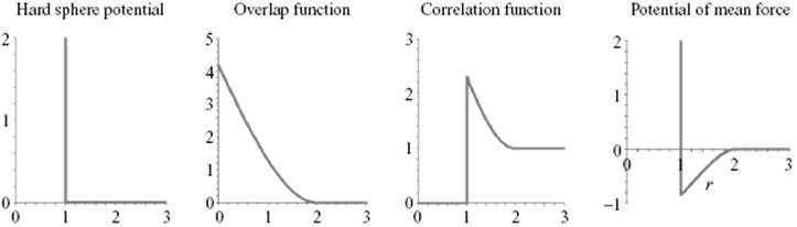
To illustrate these concepts, let us apply them to a hard-sphere fluid with a potential given by Figure 6.12.

(6.67)

Figure 6.12 The hard-sphere potential ϕ_HS, the overlap function A_HS, the correlation function g_HS and the potential of mean force W_HS as a function of r in units σ.

c6-fig-0012

Hence, we have

(6.68)

(6.69)

The function A₂₁(r) deviates from zero only if both f(r₁₂) ≠ 0 and f(r₂₃) ≠ 0 and for a hard-sphere fluid represents the volume of penetration of two spheres of radius σ/2 at distance r. Stereometry learns that this overlap function, labeled A_HS, reads (Figure 6.12)

(6.70) 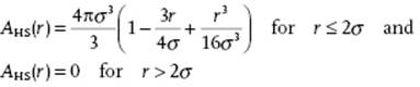c6-math-0070

This implies that the correlation function g_HS(r) for hard-sphere fluid becomes

(6.71)

representing exp(−βϕ_HS). The second factor in Eq. (6.71) results in a peak in g_HS(r) (Figure 6.12). The potential of mean force correlation W_HS(r) = −kT lng_HS(r) reads

(6.72)

The net result is an effective attractive force for σ < r < 2σ (Figure 6.12). This attraction is thus purely a result of geometric restrictions. Since⁴⁾ d exp(−βϕ_HS)/dr = −β exp(−βϕ_HS)dϕ_HS/dr = β exp(−βϕ_HS)δ(r−σ), the pressure P, given by Eq. (6.59), becomes

(6.73)

with η = πσ³ρ/6 the packing fraction⁵⁾. By using Eq. (6.66), we obtain B₂ = b ≡ 2πσ³/3 and B₃ = 5b²/8; these results have already been derived in Chapter 5.

From Example 6.1 it becomes clear that the hard-sphere correlation function is not just a step function, as one might expect naively (Figure 6.5), but rather shows an increased value near the reference molecule by the geometric restrictions imposed on the coordination shell, leading to an effective attraction. Briefly summarizing, the correlation function g(r) on average should yield a value of 1. Since g(r) = 0 for r < σ, there should be a region where g(r) > 1. Because the potential of mean force W(r) = −kTlng(r), the region where g(r) > 1 leads to W(r) < 0.

Problem 6.8*

Check the steps necessary to obtain Eqs (6.63) and (6.65).

Notes

1) Remember that we use the word “molecule” as a generic term for atoms, ions, and molecules.

2) More formally, we require translational invariance, i.e. ρ⁽¹⁾(r₁) = ρ⁽¹⁾(r₁ + r₁′) for any r₁′ (obviously not too close to the wall). This is only possible if ρ⁽¹⁾ = C with C a constant. Since we have on the one hand ∫ρ⁽¹⁾(r)dr₁ = N, and on the other hand ∫ρ⁽¹⁾(r)dr₁ = C∫dr₁ = CV, we obtain CV = N or ρ⁽¹⁾ = N/V.

3) Also known as cavity function, as it describes the distribution of cavities in a hard-sphere fluid. Note that taking logarithms results in ln g(r) = −βϕ(r) + ln y(r) or ln y(r) = ln g(r) + βϕ(r) or ln y(r) = −β[W(r) − ϕ(r)] = ΔW(r). Here, ΔW(r) represents of the potential of mean force in excess over the interaction potential ϕ(r). This permits the expansion y(r) = exp[ΔW(r)] = 1 + ΔW(r) + ½[ΔW(r)]2 + … .

4) Note that because dh(r − r′)/dr = δ(r − r′), we have dϕ_HS(r − σ)/dr = −δ(r − σ). Moreover, note that direct integration of Eq. (6.39) cannot be done because g_HS(r) is discontinuous at r = σ but can be done using Eq. (6.59) since y(r) is continuous at that point.

5) The abbreviation g(σ⁺) is defined by g(σ⁺) ≡ lim_r_→σ+0 g(r), implying that r approaches σ from the positive side. Often, g(σ⁺) is given as g(σ).

References

1 de With, G. (2006) Structure, Deformation and Integrity of Materials, Wiley-VCH Verlag GmbH, Weinheim. This book provides a concise discussion on the structure, binding and defects of solids.

2 (a) Bernal, J.D. (1964) Proc. R. Soc. A280, 299; (b) Frost, H.J. (1982) Acta Metall., 30, 889.

3 Finney, J.L. (1970) Proc. R. Soc. A319, 279.

4 Coppens, P. (1997) X-Ray Charge Densities and Chemical Bonding, Oxford University Press.

5 Pings, C.J. (1968) X-Ray Charge Densities and Chemical Bonding (eds H.N.V. Temperley, J.S. Rowlinson, and G.S. Rushbrooke), North-Holland, Amsterdam, p. 389.

6 (a) Bernal, J.D. and Mason, J. (1960) Nature, 188, 910; (b) Bernal, J.D., Mason, J., and Knight, K.R. (1962) Nature, 194, 957; (c) For further elaboration, see Bernal, J.D. (1964) Proc. R. Soc., A280, 299.

7 (a) Scott, G.D. (1960) Nature, 188, 908; (b) Scott, G.D. (1962) Nature, 194, 956.

8 (a) Woodcock, L.V. (1971) Chem. Phys. Lett. 10, 257; (b) Woodcock, L.V. (1972) Proc. R. Soc., A328, 83.

9 Eisenstein, A. and Gingrich, N.S. (1942), Phys. Rev., 62, 261.

10 Yarnell, J.L., Katz, M.J., Wenzel, R.G., and Koenig, S.H. (1973) Phys. Rev., A7, 2130.

11 Yogi, T. (1995) J. Phys. Soc. Jpn, 64, 2886.

12 Dore, J.C. (1990) Il Nuovo Cimento, 12D, 543.