Liquid-State Physical Chemistry: Fundamentals, Modeling, and Applications (2013)

8.3. Hole Models

One way to improve on the cell model is to release the requirement that each cell is always occupied by only one molecule. If we take the number of cells M somewhat larger than the number of molecules N, the volume per cell V/Mand the volume per molecule V/N become different. Accepting still maximally one molecule per cell, the empty cells are addressed as holes and the whole results in hole models [17]. Taking instead of holes, molecules of another type, the approach is also used for mixtures.

We recall that the interparticle pair potential essentially contains a repulsive part and an attractive part. The structure of a simple liquid appears to be largely determined by the repulsive part, while the attractive part mainly provides the “internal pressure,” that is, the cohesion. In order to be able to calculate the Helmholtz energy in the thermodynamic limit, the pair potential must be more repulsive than 1/r^3+δ for r → 0 and decay more rapidly than for r → ∞, where δ and δ ′ are positive constants. A simple, but nevertheless useful, model which takes both of these interactions and conditions into account is the lattice gas model. The basic concept is that the volume available to the fluid is divided into cells of molecular size. Usually, for simplicity, the cells are arranged in a regular lattice with coordination number z, for example, a simple cubic lattice with z = 6, a body-centered cubic lattice with z = 8, or a face-centered cubic lattice with z = 12. Although not required in principle, normally these cells are occupied by one particle at most, representing repulsion, and only nearest-neighbor cell attractive interactions are considered. The precise position of a particle in the cell is considered unimportant, so that the particle and cell positions are the same.

If we position N₁ molecules of type 1 and N₂ molecules of type 2 on a lattice, there will be N₁₁ (N₂₂) nearest-neighbor pairs 1-1 (2-2) of molecules of type 1 (2). Similarly, we will have N₁₂ pairs of the type in which a molecule of type 1 and type 2 combines to a pair 1-2. For any such a lattice some general relations exist. Drawing a line from each site occupied with a molecule of type 1 to the z neighboring sites, we will obtain zN lines. If the pair is of type 1-1, there will be two lines between the sites, whereas if it is of type 1-2 there is only one line. A similar consideration applies for type 2-2. Therefore,

(8.37)

Consequently,

(8.38)

If we mix N₁ molecules of type 1 with N₂ molecules of type 2, the energy is

(8.39)

The quantity w ≡ ε₁₂ − ½ε₁₁ − ½ε₂₂ is often denoted as the interchange energy. Now, we have to distinguish between a mixture of molecules of type 1 and 2 (assuming that no holes are present in the mixture) and a pure liquid with molecules (type 1) and holes (type 2). In the former case, the contribution ½ε₁₁N₁ + ½ε₂₂N₂ is a constant given by the composition, but in the latter case it is variable as the number of holes depends on the temperature. Hence, formally, we must use the canonical ensemble for the former situation describing solutions, and the grand canonical ensemble for the latter situation describing pure fluids.

8.3.1 The Basic Hole Model

We consider here the pure liquid⁴⁾ for which ε₁₁ = ε and ε₁₂ = ε₂₂ = 0, so that w = −½ε₁₁ = −½ε_. The energy E for lattices with M sites occupied by N molecules creating zX type 1-2 pairs becomes

(8.40)

The last form is somewhat more convenient in calculations. The configurational partition function becomes, using the abbreviation x = exp(−zβw) = exp(½βzε),

(8.41)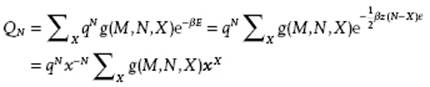

Here, q is the partition function of the molecules, assumed to be separable, and g(M,N,X) denotes the number of configurations with N molecules over M sites having X pairs of type 1-2 all having the same energy (degeneracy factor). The summation Σ_X is over all possible configurations having X pairs. Recalling the activity λ = exp(βμ) with μ the chemical potential, the grand partition function, with as usual P the pressure and V the volume, reads (see Chapter 5)

(8.42)

We will use here PV = (Pv₀)·(V/v₀) ≡ Φ·M, where v₀ is the volume of a cell and M the number of cells. Hence, Φ is the pressure in energy units.

(8.43)

(8.44)

This is as far as we can go without approximation. An exact solution is only known for 2D lattices, and therefore we have to approximate for the 3D case. The zeroth approximation (see Appendix C) considers all molecules as distributed randomly over all sites in spite of their nonzero interaction. This implies that we use the approximation

(8.45)

where the last step can be made because the summation of g(M,N,X) over all possible configurations X equals the number of configurations of N molecules over M sites. In this approximation we also have zX = N·z(M − N)/M = zN − zN²/M, leading together to

(8.46)

This sum is difficult to evaluate and we use the maximum-term method (see Justification 5.5). Denoting the terms in Eq. (8.46) by t_N, we thus approximate the sum by its maximum term⁵⁾ t_max, obtained by solving ∂t_N/∂N = 0 or, equivalently, ∂ln(t_N¬)/∂N = 0. After some algebra we obtain, using the density ρ = N/M,

(8.47)

Substituting the solution in the expression for the pressure Φ, obtained from βΦM = lnΞ = lnt_max, the result is again after some algebra, the EoS:

(8.48)

Dependent on the temperature T, the pressure Φ shows either continuously increasing curves with increasing density ρ, or sinuous curves indicating the presence of a critical point associated with a discontinuous phase transition (see Chapter 16). One phase is the more condensed and considered as the liquid with density ρ_L, while the other phase is the less dense and considered as the gas with density ρ_G. The critical point T_cri can be found by realizing the symmetry between vacant and nonvacant cells. In the two-phase region ρ_G + ρ_L = ρ, and therefore by symmetry T_cri must be at ρ_L = ρ_G = ½. The location of T_cri can now be found from ∂(βΦ)/∂ρ = 0 evaluated at ρ = ½, leading to

(8.49)

Although the basic physics of the liquid–gas transition described are qualitatively correct, the numerical accuracy is, as we will see shortly, not astonishing. In Chapter 11 and Appendix C an approximate solution based on the distribution of independent pairs of molecules (instead of independent single molecules) is briefly discussed. This solution is called the first (or quasi-chemical) approximation. In this approximation zε/kT_cri = 2z ln[(z−2)/z], so that the result for a square 2D lattice with z = 4 is zε/kT_cri = −5.54, while the exact result is zε/kT_cri = −7.05.

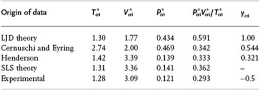
For a pure liquid we estimate, as before using the close-packed lattice, z = 12. Furthermore, in order to mimic results of other models using the LJ potential, we employ this potential here also, and take the minimum LJ potential as the value for ε and the position of the minimum r₀ = 2^1/6σ for size. We need also an expression for the partition function q and take it conform the cell model as q = v_f/Λ³ (including kinetics). In principle, v_f should depend on the local configuration, that is, the number and arrangement of nearest-neighbors. However, here we assume that we can use the value for z = 12 and discuss an improved model later. For the , we can use either the result of the zeroth or the first approximation. Employing the latter model [17], we use zε/kT_cri = 2z ln[(z − 2)/z] (see Appendix C) and obtain T_cri = −2.74ε/k. From the associated EoS and the critical volume v_cri = 2σ³, one can also calculate that P_criσ³/ε = −0.469, and therefore P_criv_cri/kT_cri = 0.342. Table 8.2 compares these results with those of the LJD and the SLS model (see Section 8.4).

Table 8.2 Critical data comparison for several theories.

So in conclusion, although the first approximation is a clear improvement over the zeroth approximation, probably the most important point to learn from the lattice gas model is that by taking the hard core seriously (no two particles on the same site) already provides the crudest approximation most of the realistic features of the liquid–vapor system, as indicated in the introduction to this Section.

8.3.2 An Extended Hole Model*

An obvious shortcoming of the simple hole model is that v_f does not depend on the local configuration, although it should. To improve this, we employ the LJD model, taking into account Kirkwood's considerations (see Justification 8.1), and write the partition function conforming with Eq. (8.36), using nearest-neighbor interactions only, so that we have with Φ_lat = ½zNϕ(0) and Ψ(r) = z[ϕ(r) − ϕ(0)]

(8.50)

Here, the communal entropy factor e^N is omitted because the idea is to incorporate this effect via a modified free volume expression.

Choosing again the FCC lattice with coordination number z₀ = 12 and cell volume a³/γ = a³/2^1/2, we assume that the coordination number becomes z = yz₀, where y is a new parameter with a range 0 ≤ y ≤ 1. Next, we define ω_k to be the fraction of vacant nearest-neighbor sites of molecule k. If all of the molecules are at the origin of their cells, we have for the potential energy of one molecule z(1 − ω_k)ϕ(0), and for the total potential energy

(8.51)

When the molecules are not at their origin, we calculate, similar to the cell model, the interaction of the wanderer with the nearest-neighbor molecule located at its origin. When the wanderer is at position r in the cell, its potential energy is Ψ(r) = z[ϕ(r) − ϕ(0)]. Using the “smearing” approximation with z(1 − ω_j) nearest-neighbors, we assume that the potential energy of the wanderer depends only on the number of nearest-neighbor molecules, and not on their precise configuration. However, this is obviously an oversimplification. Accepting this we obtain for the potential energy, using an overbar for Ψ_j to indicate the smearing approximation,

(8.52)

This results for the configurational partition function Q_N in

(8.53)

with the generalized free volume

(8.54)

When no nearest-neighbor molecules are missing (ω_k = 0), j(ω_k) becomes the same as for the cell model using the “smearing” approximation. When all nearest-neighbor molecules are missing (ω_k = 1), j(ω_k) becomes the cell size. At high and low density we obtain, respectively,

(8.55)

While the first expression is just the Einstein approximation for the partition function of a crystal, the second expression contains the factor e^N, necessary to obtain the ideal gas limit. In principle, the communal problem is thus avoided.

To calculate Q_N it is necessary to use a simple relationship for j(ω). From Eq. (8.52) we see j(ω) at T yields the same value as v_f at T/(1 − ω). We thus may use v_f = v_f(T/(1 − ω) to calculate j(ω). From Q_N, the thermodynamic properties can then be calculated in the usual way. Since v_f depends on the number and the arrangement of holes, the relationship between v_f and y is not simple [18]. Some calculations have been made with a linear approximation to ln j(ω). A comparison of the results obtained teaches us that the results are not significantly better than for the original, simpler approach.

A reasonably successful approach is based on the idea that in a fluid it is plausible to have both solid-like and gas-like molecules. If the free volume of a gas-like molecule, that is, with all its neighboring sites empty, is given by j(1) and the free volume of a solid-like molecule, that is, with all neighboring sites occupied, is labeled j(0), we may reasonably take for the average free volume, along with Henderson [19],

(8.56)

where the probability to have solid-like and gas-like properties is y_i and 1 − y_i, respectively. If we choose for the potential ϕ the LJ potential with parameters ε and σ, the expression for ϕ(0) for the FCC lattice becomes

(8.57)

where v_* = v/σ³ for the FCC lattice with intermolecular distance a and volume v = a³/2^1/2. If ω = V/M and v = V/N, we have y_i = N/M = ω/v, and the Helmholtz energy F = −kTlnZ_N evaluated using the zeroth approximation reads

(8.58)

The volume per cell is then determined by (∂F/∂ω)_V,T = 0, while the EoS can be calculated from PV = −v(∂F/∂v)_ω,T which yields, after some algebra,

(8.59)

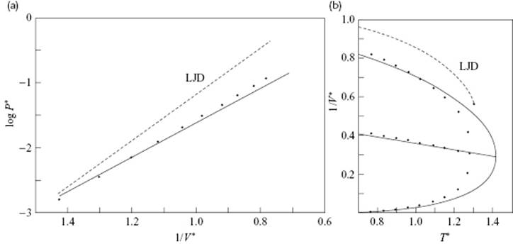
The values for j(0) and its temperature derivatives needed for a numerical evaluation can be calculated from tabulated data as given Wentorff et al. [20]. Figure 8.4 shows the vapor pressure and the EoS for the extended hole theory as calculated by Henderson in comparison with LJD theory results, and a clear improvement can be noted. Table 8.2 presents a comparison of the critical data with the results from some other theories. From these data it is clear that, for the prediction of critical constants, the simple hole theory is inferior to the LJD theory, although the extended hole theory actually represents the experimental data quite well. Henderson [19] also calculated the internal energy, entropy and heat capacity with this model, but the results obtained were inferior to those for the EoS, the reasons for which were discussed by Henderson.

Figure 8.4 Hole theory results. (a) The logarithm of the reduced vapor pressure P* for simple liquids versus reciprocal reduced temperature 1/T*; (b) The reduced density versus 1/V* versus reduced temperature T* for the hole theory (T = (ε/k)T*, V = (N/σ³)V* and P = (ε/σ³)P*). The solid line represents hole theory results, the dots represent points from the empirical Guggenheim expressions (see Chapter 4), and the dotted line represents LJD results.

In conclusion, although hole models are capable of catching the qualitative aspects of liquids correctly, and the communal problem is avoided (in principle, at least), their ultimate success is restricted. For further details we refer to the literature.

Problem 8.7

Calculate the critical constants using the simple hole theory.