An Example: Ammonia - Modeling the Structure of Liquids: The Simulation Approach - Liquid-State Physical Chemistry: Fundamentals, Modeling, and Applications (2013)

Liquid-State Physical Chemistry: Fundamentals, Modeling, and Applications (2013)

9. Modeling the Structure of Liquids: The Simulation Approach

9.4. An Example: Ammonia

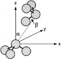
In this section we provide, as an example of the results that can be obtained using simulation methods, a means of determining the structure of liquid NH₃. This is achieved by discussing the results of combined quantum-mechanicalcalculations, pair potential fitting and MC simulations, as described by Hannongbuo [11]. In this investigation the interaction between NH₃ molecules was obtained using HF-TZP calculations⁷⁾ yielding a total energy for the molecule of −56.21603 Hartree and a dipole moment of 1.87 D. The latter value must be compared with other theoretical (quantum) calculations (Table 9.1), from which a dimer stabilization energy E_stab = −2.53 kcal mol⁻¹ was obtained with an optimum N–N distance of 3.4 Å and an optimum configuration α = β = 12°, where the angles are indicated in Figure 9.4. The interaction energy between two NH₃ molecules was calculated for more than 1500 configurations, leading to a detailed energy landscape. For ease of further calculation, this energy landscape for the NH₃–NH₃ interaction was fitted with pair potentials to these configurations. This resulted in

where the units are ΔE [kcal mol^–1] and r [Å].

Table 9.1 Dipole moments for NH₃ calculated by various approximate Hartree–Fock (HF) calculations.

c9-tbl-0001

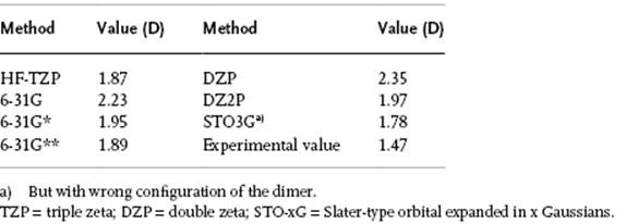
Figure 9.4 The general orientation for two NH₃ molecules with optimal configuration α = β = 12°.

c9-fig-0004

MC calculations were performed using 202 rigid NH₃ molecules with the experimental structure as described by NH = 1.0124 Å and H–N–H = 106.67°. The simulations were made at an experimental density ρ = 0.633 g cm⁻³ at 277 K, which renders a box length of 20.99 Å.

These MC simulations were first made using ab initio HF-TZP calculations for each configuration. Although a logical choice for the cut-off value would be 10.45 Å, a value of 7.0 Å was chosen because the interaction almost disappears after 5–6 Å; the computing time was also reduced. Within a shell of 7 Å this implies a calculation for about 30 molecules. The MC simulations were also made with the fitted pair potential, but in this case an expected cut-off value of 10.45 Å was used.

The N–N pair correlation function g(r) was calculated using 50 000 configurations for both (ab initio and pair potential fitted) energy landscapes, and compared with the experimental data of Narten [12] at 277 K and 1 atm. These results are shown in Figure 9.5, where the inset shows also the results for 25 000 configurations. The shape is typical for g(r). The first peak (∼3.4 Å) corresponds to the nearest-neighbor N–N distance. For the ab initio simulations a broad shoulder between 4.0 and 4.8 Å is observed, the absence of which for the pair potential simulations is attributed to a systematic error due to using simple analytical functions to represent the complicated energy surface. In particular, it was noted that for the ab initio simulations multiple minima were obtained with slightly different stabilization energies. The three most stable energies were for α = 0° with E_stab = −2.40 kcal mol⁻¹, α = 10° with E_stab = −2.53 kcal mol⁻¹, and α = 20° with E_stab = −2.25 kcal mol⁻¹ for the optimum N–N distance of 2.54 Å. For comparison, recall that RT ≅ 0.6 kcal mol⁻¹. The pair potential fitting is unable to represent these minima.

Figure 9.5 The N–N pair correlation for NH₃ as calculated from 50 000 configurations. The inset shows the results for 25 000 configurations.

c9-fig-0005

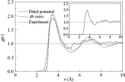
The onset of the ab initio N–N g(r) at 2.3 Å, which starts earlier than the 2.7 Å X-ray value for the experimental N–N g(r), indicates less repulsion at short distances for the pair interaction derived from ab initio calculations during the simulation than in reality, where many-body effects are present. Another source of error which leads to discrepancy between the experimental and simulated results is the use of a fitted, nonpolarizable potential in the liquid phase simulations. It has been reported that variation of the pair potential, due to the addition of higher multipoles and of the polarization effects, influences the liquid structure by changing the dimer configurations corresponding to the local maxima of the correlation functions.

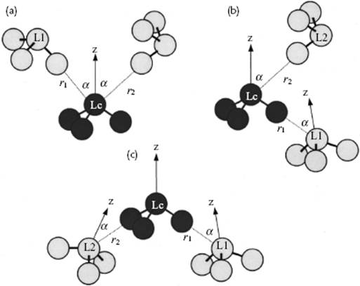
In order to investigate three-body interactions, calculations were made for the configurations as shown in Figure 9.6. The three-body contribution appeared to be important, and three configurations could be discerned within the range r₁ ≤ 2 Å and r₂ ≥ 10 Å. The configurations shown in Figure 9.6 can be described as donor–donor, donor–acceptor, and acceptor–acceptor, respectively. The donor–donor configuration appeared to be repulsive, while the donor–acceptor configuration was attractive, and the acceptor–acceptor configuration was strongly repulsive. At a N–N distance of 3.4 Å, the energy values for the donor–donor, acceptor–acceptor, and donor–acceptor configurations of 0.13, 0.65 and −0.22 kcal mol⁻¹, respectively, led to a net effect for the E_3bd value of 0.36 kcal mol⁻¹, which equates to 14% of the global minimum of the pair interaction of 2.53 kcal mol⁻¹. This influence is more pronounced for shorter distances because the three-body energy for the acceptor–acceptor increases much faster than for the other two terms.

Figure 9.6 (a) Donor–donor, (b) donor–acceptor, and (c) acceptor–acceptor configurations for three NH₃ molecules.

c9-fig-0006

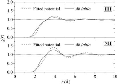
The partial pair correlation function for H–H was rather featureless (Figure 9.7), whereas the N–H correlation showed a main peak at 3.751 Å and a wide hump from 2.3 to 3.11 Å, indicating very weak hydrogen bonding in liquid ammonia. The calculated H coordination number was 0.97, compared to 1.2 from previous simulation results and 1.2 from experimental data. It should be noted that the hydrogen bond distance in solid ammonia is 2.35 Å, with an average of three hydrogen bonds per nitrogen atom.

Figure 9.7 The H–H and N–H correlation functions for NH₃.

c9-fig-0007

Overall, the remaining discrepancies between simulations and experimental can be attributed to statistical error, due mainly to the use of simple analytical functions to represent the complicated energy surface, together with many-body and the polarization effects.

Problem 9.4

Estimate the value for the average angle β from the N–N and N–H correlations functions given in Figures 9.5 and 9.7.

Notes

1) See footnote 4, Chapter 8.

2) Recall the notation introduced in Chapter 1: if a vector x is represented by a column matrix x, the inner product x·y is written as x^Ty and the set x₁x₂…x_N (x₁x₂…x_N) is represented as x (x).

3) Proper random generators are nowadays standard available for any computer.

4) See, for example, Frenkel and Smit [6].

5) Whilst for a small number of dimensions, a systematic sampling of space is more efficient, for a high number of dimensions random sampling is more efficient.

6) Whereas, in the MD method, a state means specified locations r₁,r₂,…,r_N and specified momenta p₁,p₂,…,p_N of the N particles, in the MC method a state means specified locations r₁,r₂,…,r_Nonly.

7) These abbreviations and those used later in the comparison for the dipole moment indicate the type of basis set used in the molecular orbital calculations: HF = Hartree–Fock; TZP = triple zeta, indicating that for each occupied valence orbital in the atom three basis functions are used, plus polarization functions, indicating that nonoccupied valence orbitals in the atom are included, DZP = double zeta, similar to TZP but using two basis functions, STO-xG = Slater-type orbital expanded in x Gaussian functions. Essentially, this label indicates the quality of the basis set used.

References

1 Wood, W.W. and Parker, F.R. (1957) J. Chem. Phys., 27, 720.

2 See Berenden (2007).

3 See Friedman (1985).

4 See Sachs et al. (2006).

5 See Allen (1987).

6 See Frenkel and Smit (1987).

7 Verlet, L. (1967) Phys. Rev., A159, 98.

8 Berendsen, H.J.C., and van Gunsteren, W.F. (1986) in Molecular Dynamics Simulation of Statistical Mechanical Systems (eds G. Ciccotti and W. Hoover), North Holland, Amsterdam, p. 43.

9 Wainwright, T.E. and Alder, B.J. (1958) Nuovo Cimento, 9 (Suppl. 1), 116.

10 Metropolis, N., Rosenbluth, A.W., Rosenbluth, M.N., Teller, E., and Teller, A.H. (1953) J. Chem. Phys., 21, 1087.

11 Hannongbuo, S. (2000) J. Chem. Phys., 113, 4707.

12 Narten, A.H. (1977) J. Chem. Phys., 66, 3117.