Liquid-State Physical Chemistry: Fundamentals, Modeling, and Applications (2013)

10.3. Dielectric Behavior of Gases

We have seen that there are two molecular contributions to the polarization. First, we have the dipoles induced by the applied field and, second, the alignment of permanent dipoles due to applied field. Let us consider each of these factors in turn.

For a dipole induced by a field E_int in an apolar molecule, we know that the induced dipole moment μ_ind is given by μ_ind = αE_int, where α is the polarizability. Lorentz showed that the internal field is given by E_int = E(ε_r + 2)/3 (see Justification 10.1). So, we obtain

(10.10)

where the molar volume V_m = M/ρ is used with M the molecular mass and ρ the mass density. It is traditional (although unfortunate) to call P_m ≡ α_effN_A/3ε₀ the molar polarization (with dimensions of volume/mole). Using this definition, Eq. (10.10) becomes the so-called Clausius–Mossotti equation

(10.11)

This equation links the microscopic terms, the polarizability α and number density N_A/V_m, to a macroscopic parameter, the relative permittivity ε_r. It will be clear that this expression can be applied to nonpolar fluids only.

For polar fluids, we need the permanent dipole moment averaged over all angular orientations, and to calculate this quantity we need the potential energy Φ of dipole moment μ in an electric field E given by

(10.12)

Note that μ = |μ| and E = |E| and x·y denotes the inner product of the vectors x and y, where θ is the angle between x and y. From statistical mechanics we learned how to calculate the average dipole moment: we first determine the Hamilton function, that is, the energy in terms of coordinates and associated momenta, and thereafter we evaluate the partition function and finally calculate the expectation value of μ. Here, we restrict ourselves to diatomic molecules, but the result is more general.⁵⁾

Recall that for a diatomic molecule containing atom 1 (2) with mass m₁ (m₂) at distance r₁ (r₂), the center of gravity is defined by m₁r₁ = m₂r₂. Hence, the bond length is a = r₁ + r₂, while the moment of inertia I is given by

(10.13)

We use polar coordinates r, θ and ϕ (see Appendix B) and calculate the kinetic energy T. For atom 1 we have the kinetic energy T₁ reading

(10.14)

and similarly for atom 2 so that the total kinetic T = T₁ + T₂ becomes

(10.15)

Denoting the momenta associated with θ and ϕ by p_θ and p_ϕ, we have

(10.16)

Expressed in momenta the (kinetic) energy becomes the (kinetic) Hamilton function with p = (p_θ,p_ϕ) and q = (θ,ϕ) reading

(10.17)

To obtain the associated element in phase space we rewrite Eq. (10.17) as

(10.18)

which is the equation of a circle with radius R. The element in phase space due to the momenta is thus given by

(10.19)

However, from Eq. (10.18) we also obtain

(10.20)

so that

(10.21)

Since the (total) Hamilton function is the sum of the kinetic part and potential part Φ = −μEcosθ, we have for the partition function of the diatomic rotator

(10.22)

(10.23)

(10.24)

where p_θ and p_ϕ have the range 0 ≤ (p_θ,p_ϕ ) ≤ ∞, and θ and ϕ have the range 0 ≤ θ ≤ π and 0 ≤ ϕ ≤ 2π, respectively. We see that Z separates into two factors where Z_T represents the free rotation and Z_Φ the influence of the electric field. This separation is general, and therefore the following applies to all molecules. Because, in the calculation of the average value the kinetic parts cancel, the average value of μEcosθ becomes

Using a ≡ βμE the average evaluates to

(10.25)

where the second line is obtained by expanding the exponentials. The function L(a) is usually referred to as the Langevin function, for which the approximation for small a is nearly always valid. Recalling that for the local field we need the directional field E_dir, the total average dipole moment is thus

(10.26)

Debye took for the directional field E_dir the Lorentz internal field E_int = E(ε_r + 2)/3. Making the same assumption and recalling that the induced dipole moment μ_ind is given by μ_ind = αE_int, the total dipole moment μ_tot becomes

(10.27)

where the effective polarizability is now α_eff = α + μ²/3kT. Combining with P = ε₀(ε_r − 1)E leads to the Debye equation, similar to the Clausius–Mossotti equation,

(10.28)

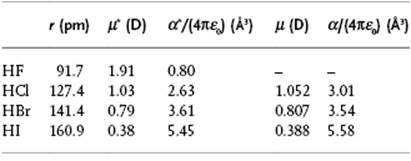
The Debye equation links the effective polarizability α_eff (and number density N_A/V_m) to the relative permittivity ε_r. A plot of P_m = V_m(ε_r − 1)/(ε_r + 2) versus 1/T yields a slope μ²/3k, while the intercept provides α. For gases, the values so obtained for the dipole moment compare rather well with independently determined values, and the method can be considered as accurate. Figure 10.1 shows the graphs and Table 10.2 the numerical data for HCl, HBr and HI as determined in this way. Figure 10.1 also shows data for the series CH₄, CH₃Cl, CH₂Cl₂, CHCl₃ and CCl₄, revealing clearly which molecules are polar and also the magnitude of dipole moment and polarizability.

Figure 10.1 Molar polarization P of (a) HCl, HBr and HI and (b) of CH₄, CH₃Cl, CH₂Cl₂, CHCl₃ and CCl₄ as a function of 1/T Data from Ref. [20].

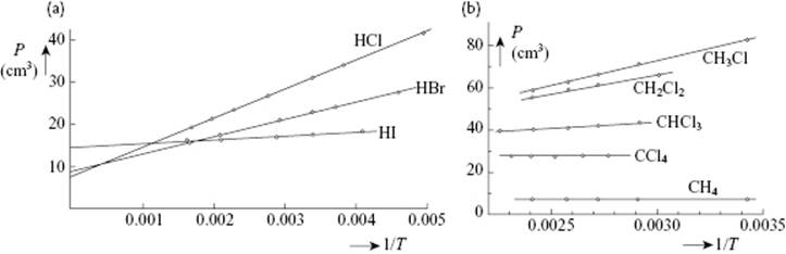
Table 10.2 Dipole moment for HF, HCl, HBr, and HI. Data from Ref. [20] and Appendix E.

So far, we have considered only the effect of a static electric field or a low-frequency electric field. With increasing frequency the polar molecules as a whole will not be able to move fast enough to comply with the field, so that the dipole orientation remains random and we are left with only the electronic polarization (Figure 10.2). According to Maxwell's equations, the refractive index n is given by n² = ε_rμ_r with ε_r and μ_r the relative electric and magnetic permittivity, respectively. Since for a dielectric μ_r = 1, we have at high frequency – that is, in the optical region – ε_∞ = n², where ε_∞ is the high-frequency relative permittivity. Hence, we can define the molar refractivity

(10.29)

which, empirically, appears to be largely independent of temperature, pressure, and state of aggregation. Equation (10.29) is conventionally addressed as the Lorentz–Lorenz equation. Note that the refractive index must be slightly temperature-dependent because of the presence of the factor V_m in the expression for R_m. For polar molecules, we thus should have R_m = P_m at high frequency. The permittivity and refractive index data for some molecules are shown in Table 10.3. It will be clear that, for the left half of the table the relationship ε_r = n² is reasonably well obeyed, but for the right half this relationship is not obeyed at all. In general this is due to cooperative effects, such as dimer formation and other structural effects, contributing to the polarization only at low frequency. Whilst in this way the effect of the electronic polarizability can estimated, the contribution of the atomic polarizability is more difficult. Böttcher [1] estimates the contribution as 5%, that is, ε_∞ = 1.05n².

Figure 10.2 Relative permittivity as a function of frequency, indicating the orientational, atomic and electronic contribution to the polarization. The dotted line indicates the loss factor.

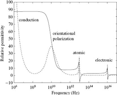
Table 10.3 Permittivity ε_r and refractive index n of several molecules.^a)

a) Data from Handbook of Chemistry and Physics (ed. R.C. Weast), 60th edn, CRC Press, 1979.

10.3.1 Estimating μ and α

One way to try to understand the dipole moment of a molecule is in terms of the contributions of the individual bonds, the so-called bond moments. As an example, consider water, the total dipole moment of which is 1.85 D, due to the vector sum of two O–H bond moments. From the total dipole moment and the geometry of the molecule, one can derive that the bond moment of an O–H bond is 1.52 D. Using this process and, on rather doubtful grounds, using a C–H bond moment of 0.4 D as a reference value, the bond moments of various bonds can be deduced. The dipole moments for several chemical bonds [2] are shown in Table 10.4, using data for saturated compounds.

Table 10.4 Dipole moments for several chemical bonds using C−H⁺ ≡ 0.4 D as a reference.^a)

a) Data calculated from methyl derivatives (CH₃X) dissolved in benzene at 25 °C.

b) Ethers, alcohols.

These data will differ for aromatic compounds as the moment of a C(sp²)–H bond differs from that of a C(sp³)–H bond. Thus, taking a value of 0.7 D for the C(sp²)–H bond, a bond moment of C(sp²)–Cl = 0.89 D from chlorobenzene can be obtained. Different authors use different values as references; for example, using C(sp³)–H = 0.31 D, C(sp²)–H = 0.63 D, and C(sp)–H = 1.05 D from infrared measurements, Petro [3] calculated C(sp³)–C(sp²) = 0.68 D from toluene (0.37 D) and propylene (0.35 D). Moreover, he obtained C(sp³)–C(sp) = 1.48 D from propyne (0.75D) and C(sp²)–C(sp) = 1.15 D from phenylacetylene (0.73 D). The problem here is that the bond contributions are considered as independent, whereas in reality the molecule should be considered as one entity of which the properties should be calculated with quantum methods.

A slightly more reliable method is to use groups of atoms in molecules. For example, in the case of nitro-groups in aromatic compounds one uses the complete nitro-group, and the dipole moment of the nitro-group in nitrobenzene replaces the dipole moment of a C–H group in the benzene molecule. In general, in this method the data are taken as the values for the monosubstituted benzenes for aromatic compounds and for monosubstituted methanes for aliphatic compounds. For further details, see Minkin et al. [2].

Similar to the dipole moment, the molar refractivity (equivalent to the polarizability) can be estimated as the sum of the contributions due to various groups in the molecule. Table 10.5 provides data for several groups from which the molar refractivity can be estimated. In contrast to the dipole moment, the estimates for refractivity (and thus polarizability) are quite accurate. Example 10.1 provides the details for both α and μ for methanol.

Table 10.5 Group contributions to the molar R_m refractivity at 589 nm.^a)

a) Data from Handbook of Chemistry and Physics, 56th edn, CRC Press, 1975.

Example 10.1: Methanol

The dipole moment μ of methanol can be estimated using the contributions of the CH₃ group (equivalent to a C–H bond), the C=O bond and the O–H bond. These contributions are, respectively, 0.4 D, 0.7 D, and 1.51·cosθ = 0.49 D with θ = 109° the C–O–H bond angle. This results in μ = 1.59 D, to be compared with the experimental value μ = 1.70 D. Whilst in this case the agreement is good, this is not always the case. The polarizability α can be estimated using the contributions of the C atom (2.591 cm³ mol⁻¹), the three H atoms (3 × 1.029 cm³ mol⁻¹) and the OH group (2.553 cm³mol⁻¹) to the molar refractivity R_m. The result is R_m = 8.23 cm³ mol⁻¹. By using R_m = N_Aα/3ε₀, one obtains α = 3.63 × 10⁻⁴⁰ C² m² J⁻¹ or α′ = α/4πε₀ = 3.26 ų, in excellent agreement with the experimental value.

Problem 10.4

Derive Eq. (10.25). Verify that L(a) ≅ a/3 for a << 1 and show that, for reasonable conditions, this approximation is nearly always satisfied. Typical values are μ = 1 D, E = 10 kV cm⁻¹, and T = 300 K.

Problem 10.5

Calculate α′ and μ for C₆H₅F given the gas-phase P_m versus T data below, and assuming ideal gas behavior.

Problem 10.6

Show that for NH₃ with an angle of 107.5° between the three N–H bonds, that is, with an angle of 68° between a N–H bond and the molecular axis through the N atom, that the bond moment is 1.31 D if the total dipole moment is 1.47 D.

Problem 10.7

Estimate μ and α′ for acetone, and compare the estimates with the experimental values μ = 2.84 D and α′ = 6.33 ų.

Problem 10.8

Given the data below, estimate the charges on the various atoms.

Problem 10.9

Indicate why R_m is expected to be largely independent of the temperature, pressure, and state of aggregation.