Liquid-State Physical Chemistry: Fundamentals, Modeling, and Applications (2013)

10.5. Water

Water is arguably the most important liquid; moreover, water behaves anomalously with respect to dielectric behavior and some other properties, and therefore deserves closer examination. We first discuss some aspects of the water molecule and its thermodynamics, and thereafter deal with some models for water, finally elaborating on the structure of liquid water and the relation of such structure to its properties.

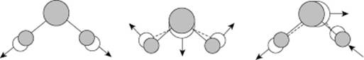
Any N-atom molecule has 3N degrees of freedom (DoF). First, there is the external motion or “rigid body” motion, which comprises translation (DoF = 3) and rotation (DoF = 3). Second, we have the internal motion of which vibration⁷⁾ is the most important. The number of internal degrees of freedom is 3N – 6 (or 3N – 5 for linear molecules). For water, we thus have three internal vibrations (Figure 10.4) that add to the value for C_P, as elaborated in Example 10.2.

Figure 10.4 The internal modes of water and their energies 3652, 1595, and 3756 cm⁻¹ (from left to right).

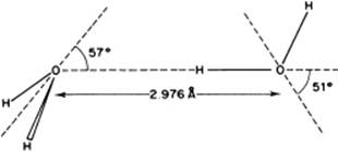
Various clusters of molecules occur in water vapor, for which theoretical estimates of bonding energy are available. For the dimer, a bonding energy of ∼22 kJ mol⁻¹ is calculated, with a rather broad minimum for the “tetrahedral” angle [8]. For the trimer, the result is a bonding energy of ∼7 kJ mol⁻¹, whilst for a quadrimer a bonding energy of ∼2 kJ mol⁻¹ is obtained. Moreover, various larger clusters seem to exist. However, taking into consideration the bonding energies mentioned, dimers are clearly the most important; the associated structure is shown in Figure 10.5.

Figure 10.5 The optimum structure of the water dimer.

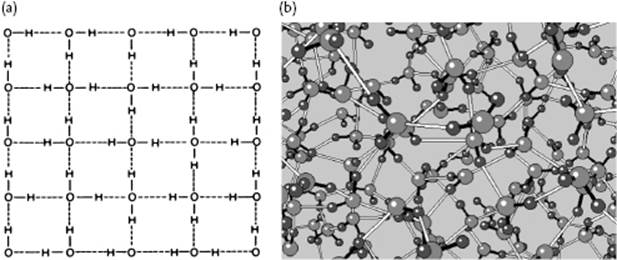
It is well known that water behaves anomalously with respect to melting: it has a negative slope for the solid–liquid transition in the P–T diagram, which implies that ice has a lower density than liquid water (Figure 10.6). On examining ice further, many polymorphs of ice exist but in our case the modification called ice I is most relevant. In the ice structure the molecules are bonded via hydrogen bonds in a tetrahedral configuration (Figure 10.7). This leads to a rather open structure that has channels, similar to diamond, and an O···O bond distance of ∼2.8 Å. Because the water molecule is almost spherical, in the lattice (almost free) overall rotations are possible. Upon cooling, one might expect that these rotations freeze out so that at 0 K the molecules would be perfectly ordered. However, it appears that ice I has a residual entropy, which indicates that at 0 K the molecules are not perfectly ordered (Figure 10.8). Pauling [9] has explained this phenomenon on the basis of the structure using the Bernal–Fowler rule, stating that each O atom is linked to four other O atoms through hydrogen bonds, twice as a hydrogen bond donor and twice as a hydrogen bond acceptor. Since N molecules have 2N H atoms and each H atom can occupy two positions, we have 2^2N configurations. For each O atom surrounded by four H atoms, we obtain 16 distinct configurations: one H₄O²⁺, four H₃O⁺, six H₂O, four HO⁻, and one O²⁻. Of these only six are used (Bernal–Fowler rule satisfied, other configurations being charged and thus less likely). The number of configurations is

and the residual entropy thus becomes, taking N = N_A,

(10.44)

Figure 10.6 The P–T diagram for water.

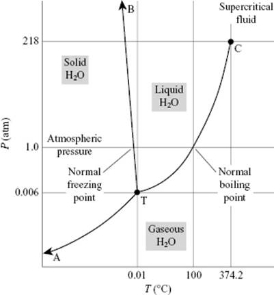
Figure 10.7 (a) The tetrahedral configuration in ice I; (b) The channels in ice I; (c) The nearly spherical shape of the water molecule. Panel (a) also shows the configuration of water as used for MC simulations. Molecules (1) and (2), as well as the central H₂O molecule, lie entirely in the plane of the paper. Molecule (3) lies above this plane, molecule (4) below it, so that the oxygen atoms (1), (2), (3), and (4) are at the corners of a tetrahedron. All distances are in Å.

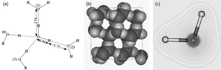
Figure 10.8 The disorder in water shown (a) schematically and (b) pictorially. The covalent O–H bonds are indicated with filled lines, while the hydrogen bonds are represented by open lines.

This value⁸⁾, characterizing the residual disorder in ice at 0 K, agrees well with the experimental data of 3.4 J K mol⁻¹ for ice and 3.2 J K mol⁻¹ for heavy ice. The residual entropy for several other molecules is estimated likewise.

Example 10.2: The entropy of water

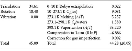
The molecular mass of H₂O is M = 18.02 g mol⁻¹, while the moments of inertia are A = 27.33 cm⁻¹, B = 14.58 cm⁻¹ and C = 9.50 cm⁻¹, and therefore θ_rot = 39.30 K, 20.96 K, and 13.7 K, respectively. The vibrational wave numbers are 3652 cm⁻¹, 1595 cm⁻¹ and 3756 cm⁻¹, so that θ_vib = 5160 K, 2290 K and 5360 K, respectively. Table 10.8 indicates the contributions from translation, rotation and vibration to the statistical entropy, as well as the experimental estimate based on the various thermodynamic processes involved. Note the limited theoretical contribution from vibration (at 25 °C, kT ≅ 200 cm⁻¹) and the relatively large experimental contribution from vaporization, as expected because of the large difference in translational motion between liquid and gas. The results imply that ΔS = 0.81 cal mol⁻¹ K⁻¹, while the Fowler–Pauling estimate yields ΔS = N_Ak ln(3/2) = 0.81 cal mol⁻¹ K⁻¹, demonstrating the good agreement.

Table 10.8 The entropy for H₂O at 298.1 K and 1 atm (all data in cal mol⁻¹ K⁻¹).

10.5.1 Models of Water

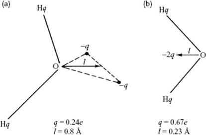
For the water molecule itself various models for the structure are available for use in calculations and simulations. These models should at least represent the dipole and local charges in the molecule. Models typically use three to five sites that may atoms or dummy sites, such as the positions of the lone pair electrons. The simplest models treat the water molecule as rigid with a geometry that matches the experimental geometry and which rely only on nonbonded interactions. The electrostatic interaction is modeled using Coulomb's law, and the dispersion and repulsion forces using the LJ potential. In particular, three-site models, using the atoms as sites, are popular in view of their computational efficiency. A simple point charge (SPC) three-site model exists with both rigid and flexible geometry. The flexible SPC model is one of the most accurate three-center water models without taking into account polarization since, in MD simulations it provides the correct density and dielectric permittivity for water [10]. Nowadays, due to increased computational power, however, more complex potentials are in use.

Early models using more than three sites were suggested by Bjerrum and Popkie (Figure 10.9). In the four-site models (Figure 10.9b), a negative charge is placed on a dummy atom near the oxygen, along the bisector of the H–O–H angle, and this improves the electrostatic distribution around the water molecule. A variety of models with the generic designation TIP4, complemented with specific labels, is currently in use. In five-site models with the generic label TIP5, the negative charge is placed on dummy atoms representing the lone pairs of the oxygen atom, with a tetrahedral-like geometry (Figure 10.9a). In particular, the TIP5P model results in a reasonably good geometry for the water dimer, a more “tetrahedral” water structure that better reproduces the experimental radial distribution functions from neutron diffraction and the temperature of maximum density of water. The TIP5P-E model is a reparameterization of TIP5P for use with Ewald sums.

Figure 10.9 The water models of (a) Bjerrum and (b) Popkie.

It should be said that a potential which describes all properties of water well does not yet exist, despite major efforts having been made. In particular, neglecting polarizability prevents an accurate description of virial coefficients, vapor pressures, critical pressure, and dielectric constant [11]. Details of many potential energy and other, more sophisticated, models are available elsewhere [12].

10.5.2 The Structure of Liquid Water

Upon melting of ice, the volume is decreased by about 9%. The heat of melting is only 13% of the sublimation energy of the solid, and this may be interpreted that a comparable percentage of hydrogen bonds rupture upon melting. Although the actual rupture percentage may be somewhat higher, since a more favorable alignment of non-nearest neighbors can occur in the liquid than in the solid, it seems safe to conclude that the majority of hydrogen bonds survive melting. In cold water, therefore, an ice-like order exists, but this disappears at higher temperature. Such disappearance can be explained by three models:

· The mixture model describing liquid water as a mixture of nonpermanent ice-like regions and fluid regions.

· The interstitial model, in which water molecules are freely moving in the empty channels of an ice-like structure.

· The distorted network model, in which an ice-like structure with distorted hydrogen bonds represents liquid water.

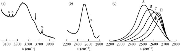
At this point, let us review the experimental data to see whether a choice can be made, or some preference can be given. The vibrational frequencies for the O–H stretching vibration are at about ∼3500 cm⁻¹ (D₂O ∼2500 cm⁻¹), while the H–O–H bending vibration occurs at ∼1600 cm⁻¹. Also librations, which represent a mixture of hindered rotation and hydrogen bond bending, occur at 300–1000 cm⁻¹. If we mix H₂O and D₂O, a rapid exchange of protons and deuterons takes place; for a mixture of 1% H₂O in D₂O, this implies that almost all of the hydrogen atoms are in HDO species. The OH stretching band for this mixture has two components, while the 1% D₂O in H₂O shows similar, though less-prominent, features for the OD stretching band. This suggests that there are two environments for the dilute isotope. The relative intensities change with temperature, and the high-frequency band is the only one present in high-density supercritical (pure) water. Only low-frequency bands are observed in ice containing both isotopes (Figure 10.10c). These features are consistent with the mixture model as well as the interstitial model. In view of the presence of two environments, the distorted model, having a wide range of configurations, seems less probable. However, in the latter model a bimodal distribution may be present, also resulting effectively in “two states.”

Figure 10.10 The Raman spectrum of (a) 1% H₂O in D₂O; (b) 1% D₂O in H₂O; and (c) the high-pressure Raman spectra of 11% D₂O in H₂O (A = 293 K, 1000 atm, B = 373 K, 1000 atm, C = 473 K, 2800 atm, D = 573 K, 4700 atm, E = 673 K, 3900 atm. In panels (a) and (b) the weak features are indicated by the arrows.

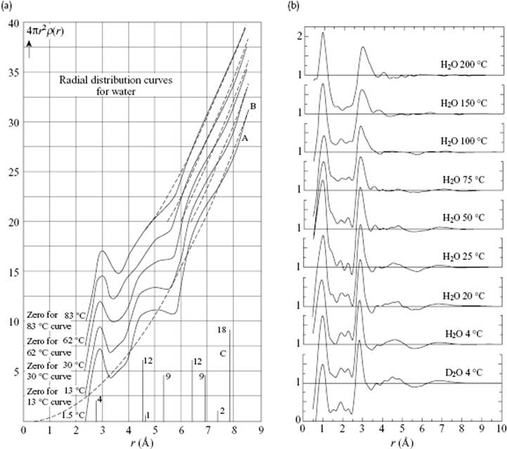
Other evidence has been provided by X-ray and neutron diffraction data of water. In Figure 10.11, the pair-correlation function for water at various temperatures, as determined by Morgan and Warren [13] and Narten and Levy [14], is shown. The scattering is mainly due to the O atoms. and only 12% results from the O···H and 2% from the H···H. The O–H bond has a length of ∼1.0 Å, while the nearest neighbor O···O distance is ∼ 2.9 Å, but this increases from 2.84 Å at 4 °C to 2.94 Å at 200 °C. These values must be compared with the distance in ice, which is 2.76 Å. The next nearest-neighbor O···O distances are ∼4.5–7.0 Å, compared to ∼4.75 and 5.2 Å in ice. Hence, the first and second neighbor distances have ice-like values, but for third neighbors the differences become appreciable. The combined diffraction evidence is strongly supportive of the persistence of tetrahedral hydrogen-bond order beyond the melting transition, but with substantial disorder present. As in the case of Ar (see Figure 6.7), the considerable improvements in experimental results over the years will be clear.

Figure 10.11 The correlation function for water at various temperatures as determined via X-ray diffraction by (a) Morgan and Warren [13] and (b) Narten and Levy [14], showing the considerable improvement in experimental data over time.

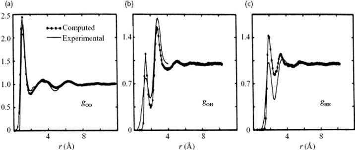
The contributions to pair correlation for water are due to the O–O distances, the O–H distances, and the H–H distances. In Figure 10.7 the basic configuration as used for a MC calculation is shown, while in Figure 10.12 a comparison is made for the partial correlation functions as obtained from this MC calculation and the experimental data. Although the latter functions are subject to interpretation, because necessarily some assumptions had to be made to distill these partial correlation functions from the total correlation function, the general agreement is good.

Figure 10.12 (a) O–O, (b) O–H and (c) H–H correlation functions resulting from MC calculations, as compared to experimental data.

An important factor for water is the presence of the hydrogen bonds. It should be stated that counting hydrogen bonds is not straightforward: their number depends on the energy criterion used. In Figure 10.13 the number of hydrogen bonds as a function of O–H···O distance is plotted for various values of the bond energy chosen. Although the distribution changes with the chosen energy level, it always shows a single peak. This renders the mixture and interstitial models less probable as they would probably result in a bimodal distribution. Computer simulations have taught us that any structural model in which there is a sharp distinction between molecules that are hydrogen-bonded and those that are not, is highly unlikely. A wide range of hydrogen bond interactions exist with no clear distinction between bonded and nonbonded molecules. Therefore, nowadays, the distorted H-bond network model is preferred.

Figure 10.13 Numbers of hydrogen bonds as a function of O–H···O distance, plotted for various values of bond energy (values shown are kJ mol⁻¹). Data from Ref. [23].

10.5.3 Properties of Water

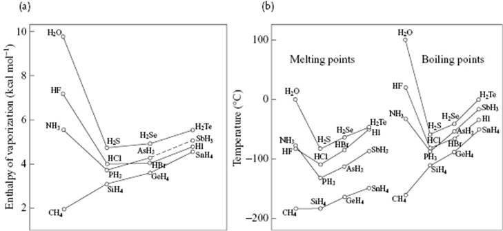
Let us now describe a few properties of water and compare the melting point, boiling point, and enthalpy of vaporization of the isoelectronic series of molecules [9] CH₄, NH₃, H₂O, and HF, all of which have 10 electrons. In this series the nuclear charge of the central atom increases from 6 to 10. At first sight, one would expect a gradual increase in properties due to increasing intermolecular interactions. Figure 10.14 shows, however, that all three properties show an extremum for H₂O. A somewhat more elaborate comparison, also shown in Figure 10.14, indicates that the three properties for a series RH_n all increase with atomic weight of R, provided that we ignore NH₃, H₂O, and HF. Extrapolating from the series SnH₄, GeH₄ and SiH₄ to CH₄ yields nearly the experimental value for CH₄ (this is also true for the series Xe, Kr, and Ar extrapolated to Ne). The corresponding extrapolation for molecules NH₃, H₂O and HF deviate, in particular for H₂O. Extrapolating the boiling point would yield about −90 °C instead of +100 °C, this deviation being due to the relatively strong intermolecular interactions. The bond energy of H₂O according to the reaction H₂O → 2H + O is 220 kcal mol⁻¹ or 110 kcal mol⁻¹ for (covalent) OH bonds.⁹⁾ Pauling has estimated the total enthalpy of sublimation of ice as 12.2 kcal mol⁻¹, and the contribution of the van der Waals interactions as one-fifth of that, leaving ∼5 kcal mol⁻¹ for a hydrogen bond. Although less than 5% of the value for the OH bond, it is the prime factor in the molecular interactions in hydrogen-bonded systems such as water. The small value Δ_fusH = 1.44 kcal mol⁻¹ indicates that only about 15% of the hydrogen bonds are broken during melting.

Figure 10.14 (a) Enthalpy of vaporization and (b) melting and boiling temperatures of isoelectronic series of hydrides, according to Pauling [9].

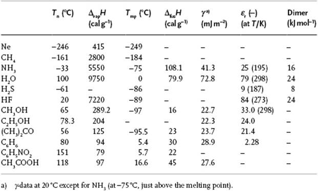
The heat capacity C_P is high and approximately constant at 1 cal g⁻¹ K⁻¹. Only C_P for NH₃ is larger, at about 1.23 cal g⁻¹ K⁻¹, due mainly to the presence of hydrogen bonds. The enthalpy of vaporization Δ_vapH is also high (Table 10.9). Notably, it takes 1 kcal to heat 1 kg of water by 1 °C, but only 2 g of water have to evaporate to cool the rest down to the original temperature (Δ_vapH = 574 cal g⁻¹ at 40 °C, about twice that for many other molecules). This is the main temperature-regulating mechanism for plants, animals and the environment, and is indeed a unique aspect of water. The enthalpy of fusion, 79.9 cal g⁻¹, is also larger than for many other molecules (except for NH₃ and a few fused salts such as KF, NaF and NaCl). For organic liquids a typical value is 45 cal g⁻¹.

Table 10.9 Properties of selected liquids.

It has already been mentioned that water expands during freezing. The density ρ of liquid water is thus higher than for ice, due mainly to the tetrahedral structure. It can be estimated that, if the H₂O molecules are treated as though they were contacting rigid spheres centered at the oxygen vertices of the lattice, the density would be only 57% of that for a close-packed arrangement of those spheres, so that a close-packed structure would result in ρ ≅ 1.75 g cm⁻³. With increasing temperature, the density increases because a fraction of the hydrogen bonds break and the molecules then occupy the vacant space. However, the kinetic energy also increases, and this leads to a lower density. Overall, water shows a maximum in density at 4 °C. The surface tension γ of water is also one of the highest (except for some liquid metals and fused salts), at about 73 mJ m⁻², compared to typical values of about 30 mJ m⁻² or less for organic liquids. In order to increase the surface area, molecules must be brought from the interior of the liquid to the surface, and the work required for this acts against the attractive forces. A similar consideration is valid for evaporation, so it is no wonder that compounds with a high Δ_vapH have also a high γ. Finally, we note that the relative permittivity ε_r, of about 80, is also higher than for many other compounds [except for liquid HCN (ε_r = 116) and formamide (ε_r = 110)], with typical values being 20 or less (compare the value for benzene, which is about 2.3). This renders the solvation capability of water for ions high, as the electrostatic forces are (very) effectively shielded. Whilst for a high value of ε_r a polar molecule is required, the cooperativity renders the permittivity of water particularly high.

Two main factors make H₂O “special”: (i) H₂O is rather polar; and (ii) the number of hydrogen atoms equals the number of lone pair electrons. This, in view of the tetrahedral arrangement, determines the extensive 3D network with a high degree of cohesion. Although the N–H···N bond is somewhat weaker than the O–H···O bond, it is more important for NH₃ that it cannot form a network but only chains and rings. Similarly, although the F–H···F bond is stronger than the O–H···O bond (even in the gas phase, HF is largely polymerized), again it can form only chains and rings. Consequently the melting point, boiling point and enthalpy of vaporization are lower than for water. Although the structure of H₂S is similar to that of H₂O, the hydrogen atoms are largely buried in the large S atom sphere, rendering the S–H···S bond very weak. Hence, the structure is close-packed rather than tetrahedral.

The question to be answered finally is: Is water unique? As with many questions in science, this question deserves a nuanced answer. When comparing some of the properties of several small molecules (as listed in Table 10.9), we see that water is not exceptionable as judged by one parameter. Rather, the anomalous behavior of water is due to the combination of several properties. Unique to H₂O is the fourfold relatively strong hydrogen-bonded coordination that is the reason for the high surface energy, permittivity, and the volume expansion during freezing.¹⁰⁾

A compact review on the structure and some properties of water has been provided by Stillinger [15], while more extended reviews are available from Eisenberg and Kauzmann [16] and in the series edited by Franks [17]. Several other aspects have been collated in a recent report [18].

Problem 10.13

At 0 °C at zero pressure, the compressibility of H₂O is κ_T = 0.51 GPa⁻¹, and reaches a minimum of 0.44 GPa⁻¹ at about 45 °C before increasing again with increasing temperature. Explain why this occurs.

Problem 10.14

Solid NO contains rectangular dimers with different side lengths. Estimate the residual entropy for NO.

Notes

1) We assume that edge effects can be neglected. We neglect also charge leakage through the capacitor.

2) We denote the polarization here by P_E to avoid confusion with the pressure P. In the remainder of this chapter we just use P for the polarization.

3) The unit of dipole moment is C m, but often the Debye unit D is used, where 1 D = 3.336 × 10⁻³⁰ C m.

4) The unit of polarizability is C² m² J⁻¹. Often, the polarizability volume α′ = α/(4πε₀) is used. Note that while α_ele represents the displacement of the electrons with respect to the nuclei, α_mol represents the displacement of the molecule as a whole.

5) For a detailed general treatment, see Ref. [19]. In brief, the Hamilton function can be written as where P are the so-called “momentoids” (pseudo-momenta) associated with the orientation angles Q used as co-ordinates while p are the momenta associated with the other co-ordinates q. This procedure separates the rigid body rotational motion, which is independent of E and therefore can be omitted. But since P are not the real momenta associated with Q, this procedure introduces a Jacobian determinant sin θ for g(Q,q,E). This is in essence the procedure used here also.

6) A detailed discussion is given by Böttcher [1].

7) For molecules containing four or more atoms other internal mechanisms may operate; for example, inversion, as in NH₃, or internal rotation, as in H₂O₂.

8) Note though that this model neglects the local topological constraints which slightly alter the statistical properties of the distribution in the neighbourhood of a site. The best series approximation for a 3D ice model yields S ≅ kln(1.5068) [22].

9) The reaction H₂O → 2H + O can be described as two consecutive reactions, H₂O → OH + H with 119 kcal mol⁻¹, and OH → O + H with 101 kcal mol⁻¹. Accordingly, the average is 110 kcal mol⁻¹.

10) Other materials that expand on freezing also have fourfold coordination, including Ga, Ge, Si, Bi, and RbNO₃.

References

1 See Böttcher (1973).

2 Minkin, V.I., Osipov, O.A., and Zhadanov, Y.A. (1970) Dipole Moments in Organic Chemistry, Plenum, New York.

3 Petro, A.J. (1958) J. Am. Chem. Soc., 80, 4230.

4 Onsager, L. (1936) J. Am. Chem. Soc., 58, 1486.

5 Kirkwood, J.G. (1939) J. Chem. Phys., 7, 911.

6 Pople, J.A. (1951) Proc. Roy. Soc., A205, 163.

7 Coulson, C.A., and Eisenberg, D. (1966) Proc. Roy. Soc., A291, 445.

8 Niesar, U., Corongiu, G., Clementi, E., Kneller, G.R., and Bhattacharya, D.K. (1990) J. Phys. Chem., 94, 7949.

9 Pauling, L. (1960) The Nature of Chemical Bond, 3rd edn, Cornell, Ithaca, NY., Ch. 12.

10 Praprotnik, M., Janezic, D., and Mavri, J. (2004) J. Phys. Chem., A108, 11056.

11 Vega, C. and Abascal, J.L.F. (2011) Phys. Chem. Chem. Phys., 13, 19663.

12 (a) Paesani, F. and Voth, G.A. (2009) J. Phys. Chem., B113, 5702; (b) Medders, G.R., Babin, V., and Paesani, F. (2013) J. Chem. Theory Comp. 9, 1103.

13 Morgan, J. and Warren, B.E. (1938) J. Chem. Phys., 6, 666.

14 Narten, A.H. and Levy, H.A. (1972) J. Chem. Phys., 55, 2263; (1972) 56, 5681.

15 Stillinger, F.H. (1980) Science, 209, 451.

16 See Eisenberg and Kauzmann (1969).

17 See Franks (1973).

18 (a) Wernet, P., et al. (2004) Science, 304, 995; (b) Zubavicus, Y. and Grunze, M. (2004) Science, 304, 974; (c) Bukowski, R., et al. (2009) Science, 315, 1249; (d) Malenkov, G. (2009) J. Phys. Condens. Matter, 21, 83101.

19 van Vleck, J.H. (1932, reprint 1966) The theory of electric and magnetic susceptibilities. Oxford, p. 32.

20 Debye, P. (1929) Polar molecules. Chemical Catalog Company.

21 Buckingham, A.D. (1967) Disc. Faraday Soc., 34, 205.

22 Nagle, J.F. (1966) J. Math. Phys., 7, 1482, 1492.

23 Rahman, A. and Stillinger, F.H. (1971) J. Chem. Phys., 55, 3366.

Further Reading

Böttcher, C.J.F. (1973) Theory of Electric Polarization, vol. 1, 2nd edn, Elsevier, Amsterdam.

Eisenberg, D. and Kauzmann, W. (1969) The Structure and Properties of Water, Clarendon Press, Oxford.

Franks, F. (ed.) (1973) Water, a Comprehensive Treatise, Plenum, New York.

Fröhlich, H. (1958) Theory of Dielectrics, 2nd edn, Oxford University Press, Oxford.

Smyth, C.P. (1955) Dielectric Behavior and Structure, McGraw-Hill, New York.