Liquid-State Physical Chemistry: Fundamentals, Modeling, and Applications (2013)

11.6. A Slightly Different Approach

So far the model has been based on mole fractions, but here we will iterate the arguments for the regular solution model in slightly different terms, that is, using the pair-correlation function [4]. From that set of arguments we will see that volume fractions are to be preferred. Other arguments in favor of using volume fractions are given in Section 11.8. The outcome leads to the solubility parameter approach, based on the Berthelot rule, Eq. (11.81), and therefore we will assess the validity of that approximation once more. Finally, it leads to the so-called one-fluid and two-fluid models of mixtures.

The argumentation starts with the energy expression

(11.86)

in which the first term represents the kinetic energy and the second term the potential energy (denoting the integral by U₀ for later reference). Furthermore, u(r) and g(r) represent the pair energy⁸⁾ and pair-correlation function, respectively. We extend this expression to a binary mixture, considering the potential energy only. In a solution around a central molecule of component 1, molecules of type 1 and 2 are found. The probability of finding a molecule of component 1 is given by (N₁/V)g₁₁(r), while the probability of finding a molecule of component 2 is given by (N₂/V)g₁₂(r). Similar relationships hold for a central molecule of component 2. Since the probabilities that the central molecule is 1 or 2 are x₁ and x₂, respectively, we may write for the total volume V, using V_α and V_m for the partial and molar volume⁹⁾ of component α and the solution, respectively,

(11.87)

(11.88)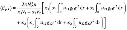

Remembering that u₁₂ = u₂₁ and g₁₂ = g₂₁, we may further simplify, meanwhile using volume fractions ϕ_i = (x_iV_i)/(x₁V₁ + x₂V₂), to obtain

(11.89)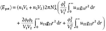

Subtracting the energy of the separate components, given by

(11.90)

we obtain for the mixing energy

(11.91)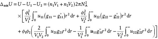

So far everything is exact, apart from the pair potential approximation. The next argument used is scaling. We use, based on the principle of corresponding states,

(11.92)

Moreover, we use the experimental similarity of g for simple molecules and write

(11.93)

in combination with σ₁₂ = ½(σ₁₁ + σ₂₂). Defining y = r/σ, we obtain for 1 mole

(11.94)

We now make the identification

(11.95)

which leads to

(11.96)

Assuming that the Berthelot approximation c₁₂ = −(c₁₁c₂₂)^1/2 is valid, we get

(11.97)

or, defining δ_α ≡ |c_αα|^1/2 = |w_αα/V_α|^1/2,

(11.98)

This expression is essentially the same as Eq. (11.56) combined with Eq. (11.81), except that mole fractions have been replaced by volume fractions. The derivation shows that the regular solution model is not necessarily based on a lattice model, but can be based on the structural analogy between solvent and solution.

11.6.1 The Solubility Parameter Approach

Hildebrand [5] introduced the solubility parameter δ_α = (ΔU_α/V_α)^1/2 so that

(11.99)

The term solubility parameter is based on the original application of the model in the solubility of compounds. Consider that miscibility occurs when Δ_mixG_m ≤ 0. Since in this model Δ_mixS_m ≥ 0 and Δ_mixH_m ≥ 0 always, Δ_mixH_mmust be not too large to result in miscibility. In other words, miscibility is predicted if w is small. Two ways to estimate δ-values exist. One way is to use the experimental enthalpy of vaporization Δ_vapH_α for the pure compounds α to calculate Δ_vapU_α = Δ_vapH_α − RT which, when combined with V_α, yields δ_α. Another approach employs group contribution methods which have been devised to estimate δ (see Chapter 13).

In order to estimate how well the geometric mean approximation for w is, we resort to the dispersion energy. Recall that in Chapter 3 an approximate expression for the dispersion interaction was given reading αβ

(11.100)

with α the polarizability and I the characteristic energy. It was indicated that estimating I as the ionization potential is doubtful, while an estimate for α is much more reliable.

Assuming , a reasonable assumption for spherical molecules, we may write from Eq. (11.95)

(11.101)

Using Eq. (11.100) for ε_αβ at r = σ_αβ and the assumption σ₁₂ = (σ₁₁ + σ₂₂)/2, we obtain

(11.102)

Because the geometric average is invariably less than the arithmetic average, the approximation c₁₂ = −(c₁₁c₂₂)^1/2 is only valid if I₁ = I₂ and σ₁₁ = σ₂₂ (as discussed in Section 3.6); otherwise, |c₁₂| < (c₁₁c₂₂)^1/2. Writing

(11.103)

(11.104)

Reed [6] estimated that for hydrocarbon + fluorocarbon systems f_I ≅ 0.97 and f_σ ≅ 0.995, rendering large deviations from the Berthelot rule using typical δ-values (this is consistent with our discussion in Section 3.6). Finally, we note that although the solubility parameter approach is empirically rather successful, its theoretical basis is flimsy.

11.6.2 The One- and Two-Fluid Model

The approach discussed provides a basis for the one-fluid and two-fluid model of mixtures. We saw that using g_αβ = g (r/σ_αβ) for all pairs of components α and β, ρ = N/V, and returning to mole fractions x_α, the configurational energy is given by

(11.105)

Using the symbols ε and σ for the mixture we can define

(11.106)

In this way a mixture can be described by a hypothetical pure, model fluid with properties defined by ε and σ given the scaled interaction and correlation functions f(y) and g(y). In the literature this model is usually referred to as the one-fluid van der Waals (or vdW1) model.

Another “Ansatz” is to use g_αβ = ½[g_αα(r/σ_αα) + g_ββ(r/σ_ββ)]. This leads to

(11.107)

(11.108)

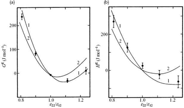
Here, g_αα represents the correlation function for a pure, pseudo-component α with ε_α and σ_α and the mixture is described as an ideal mixture of two pseudo-components. It is referred to as the two-fluid van der Waals (or vdW2) model. Although it is difficult to discriminate between the vdW1 and vdW2 models on an experimental basis, simulations using the Lennard-Jones potential clearly show that the vdW1 model is better [7] that the vdW2 model (Figure 11.6). The expressions for F and G in the vdW1 model read

(11.109)

(11.110)

respectively, where F₀ and G₀ correspond to U₀. For the vdW2 model, these expressions must be summed over the components using the appropriate values for ε and σ. In contrast to the vdW2 model, the vdW1 model introduces no ambiguities between F and G, which makes it also preferable. Since for mixtures, P and T usually are the normal variables, the use of G is more convenient.

Figure 11.6 (a) Excess Gibbs energy of mixing and (b) excess enthalpy of mixing for an equimolar mixture of 6 : 12 molecules for which σ₂₂/σ₁₂ = 1.06 at 97 K and P = 0 (ε₁₂ = 133.50 K, σ₁₂ = 3.596 Å). The points give the simulation results, and the curves marked 1 and 2 give the results of the vdWl and vdW2 theories, respectively.