Liquid-State Physical Chemistry: Fundamentals, Modeling, and Applications (2013)

In solutions in many cases ions are involved, which we discuss in this chapter. First, we deal with the solubility of salts and the thermodynamic reasons involved, followed by models and facts about hydration. Next, the Debye–Hückel theory is introduced leading to (approximate) thermodynamic expressions for ionic solutions. Thereafter, we discuss electrical conductivity, including the effect of ion pairing.

12.1. Ions in Solution

The existence of ions in solutions was not immediately clear. Following the demonstration of electrolysis by Michael Faraday (1791–1869), an important step was taken by Svante Arrhenius (1859–1927) who postulated the existence of ions in his thesis, for which he eventually received the Nobel Prize – though not after considerable debate. Other important contributions, in particular related to conductivity, were made by Friedrich Wilhelm Georg Kohlrausch (1846–1910) and Friedrich Wilhelm Ostwald (1853–1932). During this era, the distinction between strong and weak electrolytes was made, with a major breakthrough being the development of a theory for the activity coefficient of strong electrolytes by Erich Hückel (1896–1980) and Pieter Debye (1888–1966); this was later refined by Lars Onsager (1903–1976) and Hans Eduard Wilhelm Falkenhagen (1895–1971). Concepts to include association in strong electrolytes were introduced by Niels Bjerrum (1879–1958).

When dealing with ionic compounds, several questions come to mind. Why do certain salts dissolve easily but others do not? Do salts dissociate completely on dissolution of the compound? What is the configuration of the solvent around a dissolved ion? With regards to the solubility question, two approaches can be advanced – analytical and energetic, respectively – and these are dealt with in the next section. Aspects of hydration structure and dissociation are discussed in Sections 12.3 and 12.4, respectively.

12.1.1 Solubility

From an analytical point of view, solubility is described by the solubility product K_sol, directly related to Δ_solG° via

(12.1)

For example, for AgCl we have the solubility product K_sol = (a_Ag) (a_Cl)/(a_AgCl) = [a_Ag] [a_Cl] ≅ [Ag⁺] [Cl⁻], with activity a_X and molarity [X] of component X. As a first reduction step we note that, according to the definition of activity of a solid, a_AgCl = 1, whilst for the second step we neglect the difference between activity and molarity. The larger the solubility product, the greater the solubility. In the example of AgCl, K_sol = 1 × 10⁻¹⁰ using concentration units (M or mol l⁻¹) so that, if there is no other source of either Ag⁺ or Cl⁻ ions, we have, using the electroneutrality condition [Ag⁺] = [Cl⁻], [Ag⁺] = 1 × 10⁻⁵ M. For the solubility product data of some common salts, see Appendix E. Once a solubility product is determined experimentally, the rest follows.

The presence of other compounds – be it one with a common ion or an acid or base – influences the solubility to a large extent. The effect of the former is called the common ion effect, while the effect of the latter, though quite important, carries no specific name. Inert ions also influence solubility by changing the ionic strength of a solution. The influence of these ions on the solubility is conventionally addressed in basic or physical chemistry courses, and we refrain from further discussion here, apart from showing some illustrative examples.

Example 12.1: The common ion effect

Suppose that we want to dissolve AgCl in a solution of 1.0 M NaCl. The molarity of Cl⁻ ions is then [Cl⁻] = 1.0 + [Ag⁺]. The concentration of [Ag⁺] is negligible as compared to [Cl⁻], so that with [Cl⁻] ≅ 1.0 we obtain K_AgCl = [Ag⁺] [Cl⁻] ≅ [Ag⁺] × 1.0 = 1 × 10⁻¹⁰. In other words, the solubility of AgCl in 1.0 M NaCl solution is 1 × 10⁻¹⁰ M.

Example 12.2: The effect of acid–base equilibria

Suppose that we want to dissolve AgOH, a weakly soluble salt, in water. For the reaction AgOH ↔ Ag⁺ + OH⁻ the solubility product K_AgOH = [Ag⁺] [OH⁻] = 1 × 10⁻⁸, while for the water dissociation H₂O ↔ OH⁻ + H⁺ the equilibrium constant reads K_H2O = [H⁺] [OH⁻] = 1 × 10⁻¹⁴. The overall reaction reads AgOH + H⁺ ↔ Ag⁺ + H₂O, with an equilibrium constant K = K_AgOH/K_H2O = 1 × 10⁻⁶.

The solubility of AgOH in a buffer of, say, pH 11 is calculated realizing that, for a buffer solution, [H⁺] and [OH⁻] are fixed. At pH 11, [H⁺] = 1 × 10⁻¹¹ and [OH⁻] = 1 × 10⁻³. Since K_AgOH = 1 × 10⁻³ [Ag⁺] = 1 × 10⁻⁸, we obtain [Ag⁺] = 1 × 10⁻⁵ M. Similarly, in a buffer of pH 7, [H⁺] = 1 × 10⁻⁷ and [OH⁻] = 1 × 10⁻⁷. Therefore, K_AgOH = 1 × 10⁻⁷[Ag⁺] = 1 × 10⁻⁸ and [Ag⁺] = 1 × 10⁻¹ M.

In pure water, [H⁺] and [OH⁻] are not fixed so that we have to solve

simultaneously. As this involves three unknowns with only two equations, we need one more equation. The charge balance requires that

Assuming that [Ag⁺] >> [H⁺], this expression reduces to [OH⁻] ≅ [Ag⁺], so that K_AgOH = [Ag⁺]² = 1 × 10⁻⁸ and [Ag⁺] = 1 × 10⁻⁴ M. From [OH⁻] ≅ [Ag⁺] = 1 × 10⁻⁴ M we calculate [H⁺] = 1 × 10⁻¹⁰ M, so that the assumption [Ag⁺] >> [H⁺] is warranted. Formally, from K_AgOH = [Ag⁺] [OH⁻] and K_H2O = [H⁺] [OH⁻]

Solving leads to

In more complex situations, the mass balance must also be invoked.

From an energetic point of view, solubility is described by the configuration change of ions upon dissolution of a salt. During dissolution, the lattice of a salt becomes disrupted and the individual ions are hydrated. As for any process, dissolution is governed by the Gibbs energy change Δ_solG, combining the enthalpy change Δ_solH with the entropy change Δ_solS. The question arises: What controls Δ_solG?

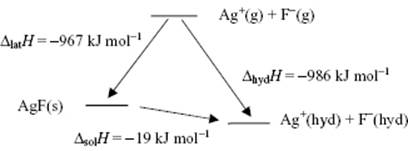
Let us first look at Δ_solH. The energetics of the dissolution process can represented by a Born diagram, similarly to the Born–Haber diagram used for lattice energies. Such a Born diagram for AgF is shown in Figure 12.1. This shows that the overall enthalpy of dissolution Δ_solH = Δ_hydH − Δ_latH = −19 kJ mol⁻¹, and that the large lattice enthalpy Δ_latH is compensated by an even larger hydration enthalpy Δ_hydH. The balance between Δ_latH and Δ_hydHdetermines whether Δ_solH < 0 (exothermic) or Δ_solH > 0 (endothermic). Since for AgF Δ_solH < 0, the liquid heats up during the process.

Figure 12.1 Born diagram for the dissolution of AgF in water, indicating the enthalpy changes.

During dissolution, heat is usually absorbed but it can also be released (e.g., for anhydrous Na₂SO₄ and CaSO₄). There can even be a change in sign of Δ_solH with temperature (e.g., for CaCl₂·2H₂O and LiCl). Within a series of compounds that are all very soluble in water, the trend may reverse: the dissolution of LiCl produces enough heat to boil the solvent, while the dissolution of NaCl produces very little temperature change, yet NH₄Cl may cool the solvent to below its freezing point.

Since both Δ_latH and Δ_hydH are large and comparable, we should also consider entropy change Δ_hydS. It appears that Δ_hydH and Δ_hydS show similar trends, for example, with ionic charge ze (z valency, e unit charge) and ionic radius a (see Section 12.2). Moreover, we should realize that ΔH and ΔS contribute oppositely to ΔG, and consequently the solubility of salts is difficult to predict. For a discussion of the dissolution trends for various salts, see Ref. [1].

The second question of whether a salt dissolves completely or incompletely into individual ions can be answered by taking measurements of the colligative properties and electrical conductivity. It appears that there are two types of electrolytes:

· Strong electrolytes showing (almost) complete dissociation, so that the colligative properties are proportional to the number of ions and the electrical conductivity is weakly dependent on the concentration.

· Weak electrolytes, with only partial dissociation, showing a strong dependence of the colligative properties and a strong dependence of the electrical conductivity on concentration.

Since we need to deal with the individual ions, we must ask also how the hydration enthalpy of one salt can be divided over the ions. It appears that the experimental values of Δ_hydH of a series of salts with common ions show approximately con­­­stant differences. For example, Δ_hydH(NaCl) = −774.6 kJ mol⁻¹ and Δ_hydH(KCl) = −690.4 kJ mol⁻¹, so that the difference is 84.2 kJ mol⁻¹. For the corresponding bromides the data are Δ_hydH(NaBr) = −740.7 kJ mol⁻¹ and Δ_hydH(KBr) = −656.7 kJ mol⁻¹, resulting in a difference of 84.6 kJ mol⁻¹, almost the same as for the chlorides [1]. Hence, if the hydration enthalpy for a single ion could be known, from a series we could calculate the enthalpies for all other ions. For this reference, the H⁺ ion is usually chosen. The choice Δ_hydH(H⁺) = 0 represents the conventional scale, while taking for Δ_hydH(H⁺) an independently determined experimental value is designated as the absolute scale. Various experimental methods to estimate Δ_hydH(H⁺), for which we refer to the literature [2], resulted in −1150.1 ± 0.9 kJ mol⁻¹ at 25 °C¹⁾. A value of Δ_hydS(H⁺) = −153 J K⁻¹ mol⁻¹ is obtained for the entropy, leading to Δ_hydG(H⁺) = −1104.5 ± 0.3 kJ mol⁻¹. In Section 12.2, we deal with a theoretical solution to the hydration question given by the Born hydration model, and with a few of its extensions in greater detail.

Problem 12.1

The solubility product of BaCO₃ is K_BaCO3 = 5 × 10⁻⁹, while the equilibrium constants for H₂CO₃ are [H⁺]/[H₂CO₃] = 4 × 10⁻⁷ and . Calculate the solubility of BaCO₃ in water.

Problem 12.2

For NaCl, which is known to dissolve well in water, Δ_latH = −788 kJ mol⁻¹, while Δ_hydH = −784 kJ mol⁻¹. What is Δ_solH ? Does the solvent cool down or heat up during dissolution? Estimate the minimum value required for Δ_solS.