Liquid-State Physical Chemistry: Fundamentals, Modeling, and Applications (2013)

In the description of liquids and solutions, we will need macroscopic and microscopic concepts that we do not consider as part of the subject proper but still are prerequisite to our topic. For macroscopic considerations, we will need phenomenological thermodynamics, and Section 2.1 presents a brief review of this. For microscopic considerations, we introduce in Section 2.2 some concepts from classical mechanics, and in Section 2.3 basic quantum mechanics and a few model system solutions. For further details of these matters, reference should be made to the books in the section “Further Reading” of this chapter, of which free use has been made.

2.1. Thermodynamics

Thermodynamic considerations are basic to many models and theories in science and technology, and in this section the phenomenological aspects of thermodynamics are briefly described but less briefly as in the summary given by Clausius [1]:

· Die Energie der Welt is constant.

· Die Entropie der Welt strebt einem Maximum zu¹⁾.

2.1.1 The Four Laws

Thermodynamics is based on four well-known basic laws²⁾. In order to describe these, we start with a few concepts. In thermodynamics the part of the physical world that is under consideration (the system) is for the sake of analysis considered to be separated from the rest (the surroundings). The thermodynamic state of the system is assumed to be determined completely by a set of macroscopic, independent coordinates a_i (also labeled a)³⁾ and one “extra” parameter related to the thermal condition of the system. For this parameter one has several choices, one of which is the most appropriate and to which we return later. Together, these constitute the set of state variables. Intensive(extensive) variables are independent of (dependent on) the size and/or quantity of the matter contained in the system. When a new set of state variable values is applied, the system adapts itself via internal processes, collectively characterized by the internal variables ξ_i (or ξ). When the properties of a system do not change with time at an observable rate given certain constraints, the system is said to be in equilibrium. Thermodynamics is concerned with the equilibrium states available to systems, the transitions between them, and the effect of external influences upon the systems and transitions [2, 3].

Depending on the problem, one assumes a specific type of wall between the system and the surroundings, that is, a diathermal (contrary adiabatic) wall allowing influence from outside on the system in the absence of forces, a flexible (contrary rigid) wall allowing work exchange, or a permeable (contrary impermeable) wall allowing matter exchange. Systems separated by an adiabatic wall are iso­lated, while systems separated by a diathermal wall are said to be closed, but in thermal contact. Finally, systems separated by diathermal permeable walls are designated as open. Sometimes the wall is taken as virtual, for example, in continuum considerations.

If any two separate systems, each in equilibrium, are brought into thermal contact, the two systems will gradually adjust themselves until they do reach mutual equilibrium. The zeroth law⁴⁾ states that if two systems are both in thermal equilibrium with a third system, they are also in thermal equilibrium with each other – that is, they have a common value for a state variable T, called (empirical) temperature. If we consider two systems in thermal contact, one of which is much smaller than the other, the state of the larger one will only change negligibly in comparison to the state of the smaller one if heat is transferred from one system to the other. If we are primarily interested in the small system, the larger one is usually known as a temperature bath or thermostat. If, on the other hand, we are primarily interested in the large system, we regard the small system as a measuring device for registering the temperature and refer to it as a thermometer.

With each independent variable a_i, often indicated as displacement, a dependent variable is associated, generally denoted as force⁵⁾ A_i. A force is a quantity in the surroundings that, when multiplied with a change in displacement, yields the associated work. Displacement and force are often denoted as conjugated variables. Work done on the system is counted positive and depends on the path between the initial and the final state. For infinitesimal changes da_ithe work δW⁶⁾ is

(2.1)

The most familiar example of work is the mechanical work δW_mec = −P dV, where P and V denote the pressure and volume, respectively⁷⁾. Other examples are the chemical work δW_che = Σ_αμ_αdn_α with the chemical potential μ_αand number of moles n_α of component α and the electrical work δW_ele = ϕ dq with the electric potential ϕ and charge q. In general, the integral over δW yields ∫δW = W, where W is not a state function, that is, a function of state variables only, contrary to the integral over a state variable a yielding ∫da = Δa. Hence, δW is not a total differential and consequently we use the notation δW instead of dW.

When work is done on an adiabatically enclosed system it appears that the final state is independent of the type of work and its process of delivery. This leads to the state function U for which we thus have dU = δW. Using other enclosures as well, the first law states that there exists a state function U, called internal energy, such that the change in the internal energy dU from one state to another is given by

(2.2)

where δQ is identified as heat entering the system⁸⁾ and interpreted as work done by the microscopic forces associated with the internal variables ξ in the system. Heat entering the system is counted as positive and also depends on the path between the two states. Although δQ and δW are dependent on the path between the initial and final states, dU is independent of the path and depends only on the initial and final states. Hence, dU is a total differential and the internal energy U a state variable which is the proper choice for the “extra”, thermal parameter of state.

Each state is thus characterized by a set of state variables a and the internal energy U. If for a process δQ = 0, it is called adiabatic. If δW = 0 we have isochoric conditions and we refer to the process involved as pure heating or cooling. If both δQ = 0 and δW = 0, the system is isolated. The first law, Eq. (2.2), can thus be stated succinctly as follows: for an isolated system, the energy is constant.

The second law states that there exists another state function S = S^(r) + S⁽ⁱ⁾, called entropy and composed of a reversible part S^(r) and irreversible part S⁽ⁱ⁾, such that for a transition between two states

(2.3)

where TdS^(r) = δQ and T is the temperature external, that is, just outside, to the volume element considered. The second law, Eq. (2.3), thus expresses that for an isolated system the entropy can increase only or remain constant at most. Since for any system the energy U is a characteristic of the state, the entropy S is a function of U and a and we write S = S(U,a). The entropy of a composite system is usually taken to be additive, that is, the sum of the entropies of the constituent subsystems, to be analytical, that is, continuously differentiable (see Appendix B), and monotonically increasing with energy. Additivity is true as long as the range of interactions between particles is small as compared to the size of the system. Conventionally, additivity is taken to imply extensivity; that is, if the extensive parameters are multiplied by λ, the entropy will obey S(λU,λa) = λS(U,a), and the entropy is thus taken as a homogeneous function of degree 1 of the extensive parameters (see Appendix B). However, this is not necessarily true but only if the effect of the interface of the system with the walls of the enclosure can be neglected. Analyticity and continuity are also not always true. For example, for a phase transition it may be impossible to express the entropy in a Taylor series around the transition temperature and it may show a jump (discontinuous transition) or a discontinuity (continuous tran­sition) in derivatives at that temperature. Normally, we accept analyticity and continuity.

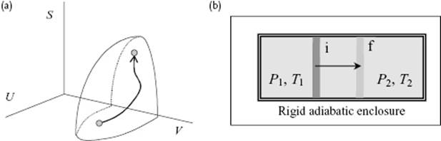
According to the second law, for a given U and a, the equilibrium state is obtained when S is maximized by the microscopic processes associated with the internal variables ξ of the system or dS(U,a) = 0 and d²S(U,a) < 0 (Figure 2.1). If the equality in Eq. (2.3) holds, the process is reversible (dS⁽ⁱ⁾ = 0), otherwise it is irreversible (dS⁽ⁱ⁾ > 0). If for a process dS = 0, it is called isentropic. If dT = 0, we refer to it as isothermal. A natural process (contrary unnatural process) is a process occurring spontaneously in Nature, which proceeds towards equilibrium and in this sense a reversible process can be seen as the limiting case between natural and unnatural processes⁹⁾.

Figure 2.1 (a) Entropy S as a function of U and V and a quasi-static process from an initial to a final state. (b) The establishment of equilibrium for an isolated system consisting of a cylinder with a frictionless piston moving from initial position i to final position f.

The entropy expressed as S = S(U,a) is called a fundamental equation. Once it is known as a function of its natural variables U and a, all other thermodynamic properties can be calculated. The description S = S(U,a) is called the entropy representation. Since S is a single valued continuously increasing function of U, the equation S = S(U,a) can be inverted to U = U(S,a) without ambiguity. For a given entropy S the equilibrium state is reached when dU(S,a) = 0. From stability considerations it follows that U is minimized by the internal processes of the system or dU(S,a) = 0 and d²U(S,a) > 0. The description U = U(S,a) is the energy representation with natural variables S and aand is also a fundamental equation. In equilibrium we have from¹⁰⁾ dU = (∂U/∂S)dS + (∂U/∂a)^Tda the (thermodynamic) temperature T = ∂U/∂S and the forces A = ∂U/∂a. From T = ∂U/∂S we easily obtain the relation T⁻¹ = ∂S/∂U. One can show that the temperature T is independent of the properties of the thermometer used, and is consistent with the intuitive concept of (empirical) temperature. The units are kelvins, abbreviated as K and related to the Centigrade or Celsius scale, using °C as unit with the same size but different origin:

(2.4)

The origin of the absolute scale, 0 K = −273.150 °C, is referred to as absolute zero.

For completeness we mention the third law, stating that for any isothermal process involving only phases in internal equilibrium

(2.5)

This relation also holds if, instead of being in internal equilibrium, such a phase is in frozen metastable equilibrium, provided that the process does not disturb this frozen equilibrium. According to the third law, absolute zero cannot be reached. The discussion of the third law contains subtleties for which we refer to the literature.

2.1.2 Quasi-Conservative and Dissipative Forces

Only for reversible systems we can associate TdS with δQ and in this case δW = Σ_iA_ida_i = A^Tda is the reversible work. For irreversible systems, TdS > δQ and the work δW contains also an irreversible or dissipative part. To show this, note that the elementary work can be written as

(2.6)

where dS = dS^(r) + dS⁽ⁱ⁾. Since U = U(S,a) we have dU = (∂U/∂S)dS + (∂U/∂a)^Tda = TdS + (∂U/∂a)^Tda. So we can also write Eq. (2.6) as

(2.7)

Therefore, the expression TdS⁽ⁱ⁾ has also the form of elementary work and we introduce forces A^(d) by writing

(2.8)

The quantity A^(d) is the dissipative force and we refer to as the dissipative work. Writing for the total force

(2.9)

we define the quasi-conservative force A^(q) by

(2.10)

which is the variable conjugated to a. Summarizing, we have

(2.11)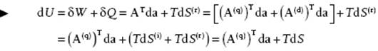

known as the Gibbs equation. The adjective “quasi-” stems from the fact that U is still dependent on the temperature while the adjective “conservative” indicates that U acts as a potential. Generally the adjective “quasi-conservative” is not added; using only the volume V for a, one refers to A = −P^(q) as just pressure and labels it as −P. We will do so likewise hereafter. Hence, in the remainder we use A_i = −P, a_i = V and write U = U(S,V) so that the pressure becomes P = −∂U/∂V. The Gibbs equation then becomes

(2.12)

However, note that in a nonequilibrium state and for dissipative processes, P = P^(q) is not the total pressure, and that in general there are more independent variables. Since for a reversible process one assumes that the system is at any moment in equilibrium, the rate must be “infinitely” slow. If this is the case the process is quasi-static. It will be clear that reversible processes are quasi-static, although the reverse is not necessarily true.

2.1.3 Equation of State

Expressed in its natural variables S and V, U(S,V) is a fundamental equation, just like S(U,V). Again, once it is known, all other thermodynamic properties of the system can be calculated. If U is not expressed in its natural variables but, for example, as U = U(T,V), we have slightly less information. In fact it follows from T = ∂U/∂S that U = U(T,V) represents a differential equation for U(S,V). Functional relationships such as

expressing a certain intensive state variable as a single-valued function of the remaining extensive state variables are called equations of state (EoS) and the intensive variable is thus described by a state function. If all the equations of state are known, the fundamental equation can be inferred to within an arbitrary constant. To that purpose we note that, since U is an extensive quantity, U(S,V) can be taken as homogeneous of degree 1 and thus, using Euler's theorem (see Appendix B), that

(2.13)

Given T = T(S,V) and P = P(S,V) the energy U can be calculated. A similar argumentation for S leads to S = (1/T)U + (P/T)V. Only in some special cases, for example, if dS(U,V) = f(U)dU + g(V)dV, the differential can be integrated directly to obtain the fundamental equation. Equation (2.13) is often referred to as an Euler equation.

Problem 2.1

The pressure is given by −P = ∂U/∂V = [∂U(S,V)/∂V]_S. Show that if one uses the equation of state U = U(T,V), P becomes

Problem 2.2

A perfect gas is defined by U = cnRT and PV = nRT, where c is a constant, n the number of moles and the other symbols have their usual meaning. Show that the fundamental equation for the entropy S is given by S = S₀ + nR ln[(U/U₀)^c(V/V₀)] with U₀ and V₀ a reference energy and reference volume.

Problem 2.3

Show, using a similar argumentation as for U, that the relation S = (1/T)U + (P/T)V holds.

2.1.4 Equilibrium

Consider an isolated system consisting of two subsystems only capable of exchanging heat (dV_i = 0). We now ask ourselves under what conditions thermal equilibrium would occur, and to this purpose we consider arbitrary but small variations in energy in both subsystems. From the first law we have dU = dU₁ + dU₂ = 0. If the system is in thermal equilibrium, since S is maximal, we must also have dS = dS₁ + dS₂ = 0. Because

(2.14)

and since dU₁ is arbitrary, we obtain T₁ = T₂ in agreement with the zeroth law. Moreover, starting from a nonequilibrium state one can show that heat flows from high to low temperature, again in agreement with intuition [3].

The procedure outlined above is in fact the general method to deal with basic equilibrium thermodynamic problems: one considers an isolated system consisting of two subsystems of which one is the object of interest and the other represents the environment. For the total, isolated system we have dU = 0. Moreover, in equilibrium we have dS = 0. Together with the closure relations – that is, the coupling relations between the displacements a_i of the system of interest and of the environment – a solution can be obtained.

Let us now consider hydrostatic equilibrium along these lines. Consider therefore again an isolated system consisting of two homogeneous subsystems but in this case capable of exchanging heat and work (Figure 2.1). For this system to be in equilibrium we write again dS = dS₁ + dS₂ = 0. However, the entropy S is now a function of U and the various values of a_i. As we are interested in hydrostatic equilibrium we take just the volume V for each subsystem. From Eq. (2.12) we obtain

(2.15)

and thus for the equilibrium configuration

(2.16)

Because the total system is isolated we have the closure relations dU = dU₁ + dU₂ = 0 and dV = dV₁ + dV₂ = 0. Therefore, since dU₁ and dV₁ are arbitrary, we obtain

(2.17)

regaining thermal equilibrium and

(2.18)

The latter condition corresponds to hydrostatic equilibrium. Hence, in hydrostatic equilibrium the temperature and the pressure of the subsystems are equal.

2.1.5 Auxiliary Functions

The Gibbs equation for a closed system is given by

(2.19)

which gives the dependent variable U as a function of the independent, natural variables S and V. From consideration of the second law, the criterion for equilibrium for a closed system with fixed composition is that dS(U,V) = 0 or Sis a maximum at constant U. Equivalently, as stated earlier, dU(S,V) = 0 or U is a minimum at constant S. Both descriptions are complete but not very practical, since it is difficult to keep the entropy constant and keeping the energy constant excludes interference from outside. Therefore, auxiliary functions having more practical natural variables are introduced.

If we write the energy as U(S,V), the enthalpy H is the Legendre transform¹¹⁾ of U with respect to P = −∂U/∂V, which is obtained from

(2.20)

After differentiation this yields

(2.21)

Combining with dU = TdS − PdV results in

(2.22)

The natural variables for the enthalpy H are thus S and P and the equilibrium condition becomes dH(S,P) = 0.

Similarly, writing H(S,P), the Gibbs energy G is the Legendre transform of H with respect to T = ∂H/∂S and given by

(2.23)

On differentiation and combination with dH = T dS + V dP this yields

(2.24)

of which the natural variables are T and P. Consequently, the equilibrium condition becomes dG(T,P) = 0. A third transform is the Helmholtz energy F, defined as

(2.25)

with natural variables T and V and the corresponding equilibrium condition dF(T,V) = 0. It is easily shown that, for example,

(2.26)

(2.27)

The functions U(S,V), H(S,P), F(T,V) and G(T,P) thus act as a potential, similar to the potential energy in mechanics, and are called thermodynamic potentials. The derivatives with respect to their natural, independent variables yield the conjugate, dependent variables. These potentials are also fundamental equations. A stable equilibrium state is reached when these potentials are minimized for a given set of their natural variables, that is, when dX = 0 and when d²X > 0, where X is any of the four functions U, H, F, or G. The advantage of using F and G is obvious: While it is possible to control either the set (V,T) or (P,T) experimentally, control of either the set (V,S) or (P,S) is virtually impossible. As an aside we note that the Legendre transform can be also applied to the entropy yielding the so-called Massieu functions. These also act as potentials, for example, X(V,T) = S − U/T or Y(P,T) = S − U/T − PV/T. It will be clear that X is related to F and Y to G. In practice, these functions are but limitedly used, although they were invented before the transforms of the energy.

2.1.6 Some Derivatives and Their Relationships

Apart from the potentials, we also need some of their derivatives, sometimes denotes as response functions, and their mutual relationships. Consider the relations

The heat capacities are defined by

It thus follows that

Three other derivatives that occur frequently are the compressibilities κ_X (X = T or S) and the (thermal) expansion coefficient or (thermal) expansivity α ≡ α_P.

Moreover, if dϕ = Xdx + Ydy is a total differential, we can use the Maxwell relations (∂X/∂y)_x = (∂Y/∂x)_y. From the expressions for dU, dH, dF and dG we obtain

which can be used to reduce any thermodynamic quantity to a set of measurable quantities. Only three of the quantities C_V, C_P, κ_T, κ_S and α are independent because

(2.28)

Using the third law, it can be shown that at T = 0, C_P = C_V = 0 and α = 0. Using the relations S = −∂F/∂T and S = −∂G/∂T, we have the Gibbs–Helmholtz equations

(2.29)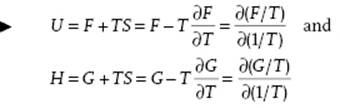

Problem 2.4

Show for a perfect gas (see Problem 2.2) that C_V = cNR, C_P = (c + 1)NR, κ_T = 1/P and α = 1/T.

Problem 2.5

Prove Eq. (2.28) and show that C_P/C_V = κ_T/κ_S.

Problem 2.6

Show that, if F = C/T where C is a constant, F = ½U.

Problem 2.7: Blackbody radiation

For blackbody radiation in a volume V the pressure P is given P = u/3 with energy density u = U/V and U(T) the total energy being a function of temperature T only. Using dU = TdS − PdV, show that u = aT⁴ where the constant a is called the Stefan–Boltzmann constant. Using (∂S/∂V)_T = (∂P/∂T)_V, show that s = S/V = 4aT³/3 yielding T and P as functions of S. Finally, show that S = CU^3/4/4V^1/4 with C = 4a^1/3/3 a constant.

2.1.7 Chemical Content

The content of a system is defined by the amount of moles n_α of a chemical species α in the system which can be varied independently, often denoted as components. A mixture is a system with more than one component. A homogeneous part of a mixture, that is, with uniform properties throughout that part, is addressed as phase while a multicomponent phase is labeled solution. A system consisting of a single phase is called homogeneous, while one consisting of more than one phase is labeled heterogeneous. Moreover, a phase can be isotropic and anisotropic (pro­perties independent or dependent on direction within a phase). The majority component of a solution is the solventwhile solute refers to the minority component. For an arbitrary extensive quantity Z of a mixture, we have the molar quantities or for a pure component α (sometimes also indicated by Z_m(α), z_α or even z when no confusion is possible). For mixtures, we also define for any extensive property Z the associated partial (molar) property Z_α as the partial derivative with respect to the number of moles n_α at constant T and P. For example, the partial volume V_α given by

(2.30)

and similarly for U_α, S_α and so on. At constant T and P we thus have

(2.31)

Since Z is homogeneous of the first degree in n_α, we have by the Euler theorem

(2.32)

Hence, we may regard Z as the sum of the contributions Z_α for each of the species α.

We note that, besides the number of moles n_α, various other quantities are used for amount of substance. We will also use the number of molecules N_α = N_An_α with N_A as Avogadro's number. Frequently, one is only interested in relative changes in composition, and to that purpose one uses the mole fraction defined by , using . In the sequel, the expressions for a binary system are given in parentheses with index 1 referring to the solvent, and index 2 to the solute.

Indicating the molar mass of the solvent by M₁, one defines the molality m_α ≡ n_α/n₁M₁ and since the mole fraction x_α = n_α/Σ_αn_α = n_α/n we have

(2.33)

For dilute solutions, n_α≠1 → 0 and we obtain m_α/x_α = 1/M₁ (m₂/x₂ = 1/M₁). If M₁ is expressed in kg mol⁻¹, the unit of molality becomes mol kg⁻¹, often labeled as m, for example, for 0.1 mol kg⁻¹ one writes 0.1 m.

In practice, molarity c_α ≡ n_α/V with V the total volume of the solution, is also used. Since ρV = Σ_αn_αM_α with ρ the mass density¹²⁾ of the solution, we have

(2.34)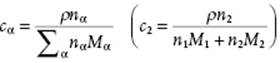

Using again the mole fraction x_α, the result

(2.35)

is easily obtained. For dilute solutions, n_α≠1 → 0 and we obtain c_α/x_α = ρ/M₁ (c₂/x₂ = ρ/M₁). If c_α is expressed in mol l⁻¹, labeled as M, one often speaks of concentration, for example, for c_α = 0.1 mol l⁻¹, one writes 0.1 M. Whatever measurement for composition is used, it is expedient to use as other independent variables P and T so that differentiation with respect to T implies constant P, and vice versa. From c_α we obtain the relation ∂c_α/∂T = −c_αα_P with α_P the expansion coefficient, and therefore c_α is not independent of temperature. This renders theoretical calculations using c_α as independent variable often cumbersome.

For chemical problems, that is, where a change in chemical composition is involved, the fundamental equation becomes U = U(S,V,n_α) or S = S(U,V,n_α). This leads to

(2.36)

The partial derivative μ_α = ∂U/∂n_α is called the chemical potential and is the conjugate intensive variable associated with the extensive variable n_α in the chemical work dW_che = Σ_αμ_αdn_α. Equilibrium is now obtained when dU(S,V,n_α) = 0.

For obtaining a potential in terms of T and V, we use a Legendre transforma­tion of U with respect to T = ∂U/∂S using the Helmholtz energy F = U − TS and obtain

(2.37)

so that F = F(T,V,n_α) and the equilibrium condition reads dF(T,V,n_α) = 0.

Applying a Legendre transformation of U with respect to T = ∂U/∂S and P = −∂U/∂V using the Gibbs energy G = U − TS + PV leads to

(2.38)

The Gibbs energy is thus given by G = G(T,P,n_α) and the equilibrium condition becomes dG(T,P,n_α) = 0. Because the chemical potential μ_α of the component α is defined as μ_α = ∂G/∂n_α, it is equal to the partial Gibbs energy G_α. Since G is homogeneous of the first degree in n_α, we have by Euler's theorem . On the one hand, we thus have

while on the other hand we know that G = G(T,P,n_α) and thus that

Therefore, we obtain by subtraction the so-called Gibbs–Duhem relation

(2.39)

implying a relation between the various differentials. This relation is here derived for T, P, and n_α as the only independent variables, but the extension to any number of variables is obvious. Moreover, although derived here for μ_α = G_α, it will be clear that a similar relation can be derived for all partial quantities.

Finally, we can also apply a Legendre transformation to U with respect to T = ∂U/∂S and μ_α = ∂U/∂n_α by using Ω = U − TS − Σ_αμ_αn_α = F − Σ_αμ_αn_α leading to

This so-called grand potential Ω is mainly used in statistical thermodynamics (Chapter 5). Since we showed that Σ_αμ_αn_α = G, we identify the grand potential as

Problem 2.8

Show that for the perfect gas (see Problem 2.2) the fundamental equation S = S(U,V,n) is given by

where u and v denote molar quantities and the subscript 0 refers to reference values. First, use the Gibbs–Duhem equation for dμ to show that the chemical potential μ is given by

Thereafter, use the Euler equation S = (1/T)(U + PV − μN).

2.1.8 Chemical Equilibrium

At constant P and constant T the Gibbs energy in a chemically reacting system varies with composition as dG = Σ_αμ_αdn_α. For a reaction to occur spontaneously dG = Σ_αμ_αdn_α < 0 while at equilibrium¹³⁾ dG = Σ_αμ_αdn_α = 0. Let us consider the reaction

(2.40)

where a, … , d denote the stoichiometric coefficients of components A, … , D. It will be convenient to rearrange this expression to

with a positive value for the coefficient ν_α when α is a product (C, D) and a negative value when α is a reactant (A, B). We define a factor of proportionality dξ(t) in such a way that dn_α = ν_αdξ . Starting at time zero with initially n_α(0) moles of each species the changes of the number of moles of each species in the time interval dt are

where is the rate of reaction. This leads to

where we introduced the affinity D = −Σ_α(ν_αμ_α). From dG ≤ 0 we conclude that

(2.41)

as the condition for a reaction to occur. So, D and must have the same sign or be zero. At equilibrium D = 0. Since ν_α = dn_α/dξ, the affinity D is related to the fundamental equations, the most important ones being, using μ_α = ∂U/∂n_α = ∂G/∂n_α = −T∂S/∂n_α,

(2.42)

All n_α must be positive or zero and the reaction goes to completion if one of the components is exhausted. This implies a lower and upper value for Δξ. Therefore, the factor Δξ is sometimes normalized according to

where ε is the degree of reaction. Writing for the chemical rate of work or power mimics the expression for the mechanical power with force A and rate of displacement . In both cases the power is positive semi-definite, that is, .

Example 2.1

A vessel contains a ½ mole of H₂S, ¾ mole of H₂O, 2 moles of H₂, and 1 mole of SO₂ and is kept at constant T and P. The equilibrium condition is

If the chemical potentials are known as a function of T, P and the n_α's, the solution for dξ can be obtained. Suppose that the solution is dξ = ¼. If dξ = ⅔, and therefore this is dξ_max. If dξ = −⅜, and therefore this is dξ_min. Therefore, the degree of reaction ε = [¼ − (−⅜)]/[⅔ − (−⅜)] = 3/5.

The above formulation leads immediately to the conventional chemical description. Let us introduce for component α the absolute activity λ_α = exp(μ_α/RT) and define, considering again the reaction given by Eq. (2.40), the reaction product

(2.43)

Using the more compact notation introduced before we write more briefly . The equilibrium condition D = −Σ_α(ν_αμ_α) = 0 can then be written as .

For solid–gas reactions we distinguish between gases (α) and solids (β). This allows us to write , where the first product contains all the terms relating to gaseous species and the second to the solid species. Now note that the chemical potential μ_α of a gaseous component α is given by , where is the chemical potential in the standard state, R is the gas constant, y_α = f_x,αx_αP is the activity (for gases often denoted as fugacity), f_x,α is the (mole fraction) activity coefficient, P is the total pressure, and P° is the standard pressure (1 bar). Hence for a gas , where is the value of λ_α for P = P°. For gases at low pressures (hence activity coefficient f_x,α = 1) the activity becomes the partial pressure P_α given by P_α = x_αP. For solids, on the other hand, we have , only weakly dependent on the pressure. In total we have

The (pressure) equilibrium constant K_P is related to the standard Gibbs energy

(2.44)

via Δμ = −RTln K_P. Since Δμ is constant at constant temperature, the value of K_P is constant at constant temperature, which explains the name. If activities are used throughout, we refer to the activity equilibrium constant K_y.

For reactions in solution we start again with and use with f_m,α the (molality) activity coefficient for molality m_α and the value for . This leads to

(2.45)

where K_m is the (molality) equilibrium constant. For ideal solutions or ideally dilute solutions m_α → 0, f_m,α → 1 and thus in that case . Similarly using with f_c,α the (molarity) activity coefficient for component α for molarity c_α and the value for leads to

(2.46)

where K_c is the (molarity) equilibrium constant. If c_α → 0, f_c,α → 1.

Problem 2.9

Derive the chemical equilibrium condition as done along the lines of hydrostatic and thermal equilibrium.