The SAFT Approach - Mixing Liquids: Polymeric Solutions - Liquid-State Physical Chemistry: Fundamentals, Modeling, and Applications (2013)

Liquid-State Physical Chemistry: Fundamentals, Modeling, and Applications (2013)

13. Mixing Liquids: Polymeric Solutions

13.6. The SAFT Approach*

After having investigated hard-sphere fluids (see Chapter 7), Wertheim focused his attention on “sticky” hard spheres in order to be able to discuss the association of molecules – that is, dimerization and polymerization [25]. Subsequently, Wertheim developed a Thermodynamic Perturbation Theory (TPT) that uses a (hard-sphere) repulsive core and one or more directional short-range attractions. In this theory, the Helmholtz energy is calculated from a graphical summation of interactions between different species (the derivation is complex and is omitted here). Wertheim's research led to the development of the Statistical Associating Fluid Theory (SAFT), as developed by Chapman and Gubbins [26] on the one hand and Huang and Radosz [27] on the other hand. Although only minor differences exist between these two developments, the Huang–Radosz development has gained more acceptance, and the present discussions are mainly limited to this approach. Although conventional EoS theories are capable of describing simple and normal liquids rather satisfactorily, their use for complex liquids often results in a description with unphysical parameter values and/or mixing rules. The reason for this is that electrostatic associative interactions (as occur in hydrogen bonding, highly polar liquids and electrolytes) are not taken explicitly into account. The basic idea of SAFT is to take association explicitly into account, where association refers to both covalent bonding (as for polymeric chains) as well as noncovalent interactions (as for hydrogen bonding). Covalent bonding is considered as a limiting case of noncovalent bonding, so that for both type of interaction Wertheim's results can be used.

In a perturbation approach, a reference fluid is chosen to which desirable properties are added. In SAFT it is assumed that the excess Helmholtz energy F^E can be composed from three major contributions to a (pair-wise additive) potential. These are: the segment contribution F^seg, representing the interaction between the individual segments; the chain contribution F^chain, due to the fact that the segments form a chain; and the association contribution F^ass, due to the possibility that some segments associate with other segments. SAFT is thus more of a framework for an EoS than a specific theory and has, therefore, led to many variants, some of which are indicated here. For the many other variants, we refer to the (review) literature [28].

Consequently, the excess (or residual) molar Helmholtz energy is given by

(13.103)

where T and ρ represent the temperature and density of the system, and the excess is defined with respect to the Helmholtz energy of the ideal gas. The segment contribution contains a repulsion and dispersion contribution, F^seg(T,ρ) = F^rep(T,ρ) + F^dis(T,ρ) = Σ_αx_αm_αF^mon, where F^mon represents the Helmholtz energy of a fluid in which the segments are not connected. The summation is over all species α with mole fraction x_α and number of segments m_α. Originally, the repulsion term was approximated by a hard-sphere (HS) contribution, expressed by the Carnahan–Starling expression, so that

(13.104)

where m is the number of spherical segments per molecule and η is the reduced density η = 0.74048 ρmv° with v° the close-packed hard-core volume of the fluid. The latter is approximated by

(13.105)

in which u° is a dispersion energy parameter per segment and C = 0.12 is a constant (except for hydrogen for which it is C = 0.241). The parameters m, v°° and u° are three parameters which are normally fitted to pure-component vapor pressure and liquid density data. In the original formulation the dispersion term F^disp is based on molecular simulation data for the square-well (SW) fluid, and reads

(13.106)

with u/k = (u°/k) (1 + βe), where e/k = 10 K for all molecules except for a few small molecules [27]. Alternatively, one uses other potentials such as the Lennard-Jones (LJ) potential, for which a closed-form EoS expression [29] is available (soft-SAFT), if necessary adding dipole–dipole interactions, possibly approximated by a Padé approximant for the perturbation expression (SAFT-LJ). As long as the EoS for the reference fluid used is known, it can be used directly.

The chain term F^chain is based on the Wertheim TPT expression to first order for association in the limit of infinitely strong bonding between infinitely small association sites. In this way, polymerization is accounted for. By using one association site per segment, one obtains a description of the thermodynamics of hard-sphere dumbbell fluids which is almost as accurate as the exact solution [25d]. Using two diametrically positioned association sites, one obtains a linear chain for which holds that

(13.107)

where y^seg is the cavity function evaluated at (bond) length l. For tangent LJ-spheres or hard spheres, the cavity function y^seg reduces to y^seg(σ) = g^seg(σ), where g^seg denotes the pair-correlation function and σ either the LJ hard-core or HS diameter. In the latter case, for a single component, Eq. (13.107) reduces to

(13.108)

The first-order theory provides a good approximation for linear chains. Bond angles are not taken in to account, although this could be done using second-order TPT though at the cost of considerable complexity. In any case, for accurate results a high-quality pair-correlation function must be used.

If we add regular association sites to the molecule, characterized as before by a non-central potential located at the edge of the molecule, one can account for association. Each of these sites can bond to only one other site located at another molecule with a single bond.⁸⁾ The detailed calculation is complex, and Justification 13.2 provides a heuristic derivation from which the association energy is given by

(13.109)

with M_α the number of association sites per species α and X_α,j is the mole fraction of species α not bonded at site j. The latter quantity is calculated from

(13.110)

where Δ_ij is the association strength evaluated from

(13.111)

where in the first part on the right-hand side, as before, g^seg is the segment pair correlation function and f_ij = exp[−βϕ(r_ij)] − 1, which is the Mayer function with ϕ(r_ij) the association potential. In the second part on the right-hand side, the SW potential is introduced with two pure-component parameters, namely the energy of association ε_ij and volume of association κ_ij. Although these parameters can be determined from spectroscopic data of the pure components, in practice they are fitted to experimental liquid density and vapor pressure data of the mixture, as are the other parameters.

For a dimerizing fluid with only one associative site per molecule, Eq. (13.109) reduces to

(13.112)

from which we obtain for the fraction monomers

(13.113)

For two association sites i and j per molecule, for example in alcohols, the oxygen lone pair and the hydroxyl proton for creating a hydrogen bond, we have

(13.114)

with still for the fraction monomers X = X_i = X_j the analytical expression as given by Eq. (13.113). For more complex models or other parameters, implicit expressions often result.

For mixtures, for the repulsion an expression for hard-spheres mixtures [30] is used. The chain and association terms can still be evaluated by the exact TPT expressions, while the dispersion terms are evaluated using the van der Waals one-fluid approximation (vdW1, see Section 11.6) reading, using x_i as the mole fraction for component i,

(13.115) 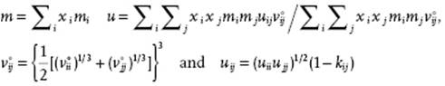c13-math-0115

where k_ij is a binary adjustable parameter for the interaction energy. Sometimes, a similar parameter is used for the hard-core volume or, equivalently, the diameter.

Summarizing so far, in SAFT a minimum of two parameters is used for each segment, namely a characteristic energy and characteristic size, and this suffices for simple conformal fluids. For non-associating chain molecules, however, a third additional parameter m characterizing the DP is required. For association, another two parameters are required, characterizing the association energy and the volume available for association for each of the interaction sites defined. All of these parameters are usually obtained from experimental data fitting, but they can also be obtained from ab initio calculations or spectroscopic information.

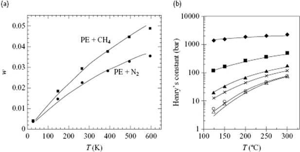
SAFT has been successfully applied to many systems, including low-pressure polymer phase equilibria. As an example, Figure 13.10 shows the solubility of CH₄ and N₂ in polyethylene, and the weight fraction Henry's law constant for various small molecules in low-density polyethylene at 1 atm, both over a wide temperature range. SAFT using a single temperature-independent binary interaction parameter provides an accurate correlation of the experimental data.

Figure 13.10 (a) Solubilities (w weight fraction of gas) of methane (upper curve) and nitrogen (lower curve) in polyethylene, as calculated from SAFT. Data from Ref. [39].; (b) Weight fraction Henry's constant of ethylene (♦), n-butane (■), n-hexane (♦), n-octane (), benzene (×), and toluene () in low-density polyethylene at 1 atm. Experimental data (points) and SAFT correlation (lines) using a single temperature-independent binary interaction parameter. Data from Ref. [40].

c13-fig-0010

Several adjustments have been made to the original SAFT model. For example, in the hard-sphere SAFT (SAFT-HS) the dispersion term is replaced by a simple van der Waals term reading βF^disp/N_A = mβu°η, meanwhile using the vdW1 rules for mixtures. This version was used (among others) to predict generalized phase diagrams for model water–n-alkane mixtures. An empirical modification is provided by replacing the hard-sphere, chain and dispersion terms by a cubic EoS (see Chapter 4) and retaining the original TPT association term (Cubic-Plus-Association, CPA). In spite of this simplification, this approach provides an accurate description of vapor–liquid equilibria (VLE) and liquid–liquid equilibria (LLE) [31]. Obviously, polarity is not explicitly included and, in spite of some semi-empirical options, a “polar CPA” is not available. The SAFT-LJ model was originally applied to water, and was further applied to pure alkanes and alcohols and to binary VLE mixtures of water, alkanes, and alcohols. The soft-SAFT model was applied successfully to pure n-alkanes, 1-alkenes, and 1-alcohols and to binary and ternary n-alkane mixtures, including the critical region. Many other modifications are discussed in the literature [24], for example, taking in account the effect of intramolecular interactions [32] and interfaces in liquid–liquid and liquid–solid systems, and its use for ionic liquids, electrolytes, liquid crystals biomaterials, and oil reservoir fluids. For these modifications, we refer to the literature [28].

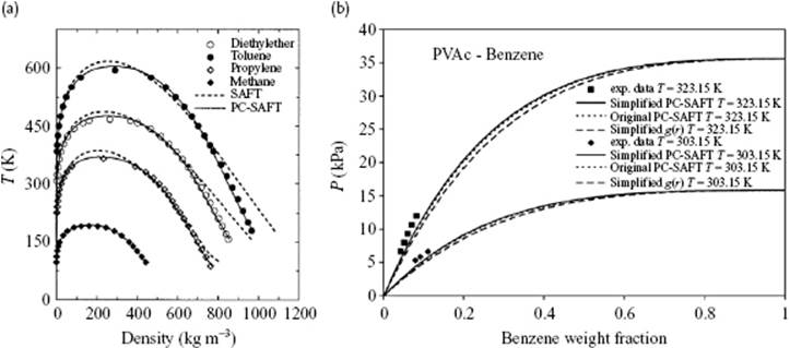
While many forms of SAFT use the hard-sphere as a reference fluid, add the dispersion term and then form chains (for polymeric solutions), in perturbed chain-SAFT (PC-SAFT) the chains are formed first and a dispersive interaction for chains is added thereafter. This implies that F^seg(T,ρ) = F^HS(T,ρ) + F^dis(T,ρ), later adding F^chain(T,ρ), is replaced by F^seg(T,ρ) = F^HS(T,ρ) + F^chain(T,ρ) and adding F^dis(T,ρ) later. Obviously, this requires a (hard-)sphere chain reference fluid. The original [33] and a simplified [34] form yield very comparable results (Figure 13.11), and in both cases only one extra energy interaction parameter k_ij is used.

Figure 13.11 (a) Saturated liquid and vapor densities for methane, propylene, diethyl ether and toluene comparing PC-SAFT (––) and SAFT (- - -) results to experimental data; (b) Comparing the vapor pressure of polyvinyl acetate (PVAc) in benzene at 303 and 323 K using PC-SAFT (···) and simplified PC-SAFT (––).

c13-fig-0011

SAFT accounts for chain connectivity rigorously, and is therefore accurate for polymers. Pure polymer EoS parameters are usually calculated by fitting melt PVT data over a wide temperature and pressure range (typically 0–200 MPa), similar to the CM, FOVE, LFT, and other models. In the case of SAFT, polymer parameters regressed from PVT data do not provide a good description of mixture phase equilibria, even with the use of large binary interaction parameters. This drawback is attributed to the use of parameter values obtained from PVT data, with parameters probably not accounting fully for the intramolecular structure, which becomes important as the molecular size increases. Similarly, intramolecular interactions become more important when the density decreases and SAFT leads to unrealistic, predicted low-density limits. On the other hand, SAFT pure-component parameters for small molecules in a homologous series vary smoothly with molecular mass and, as a result, they can be extrapolated to high-molecular-mass values and used for mixtures containing heavy oil fractions or polymers.

In conclusion, SAFT-based models have received an impressive acceptance in both academia and industry as the leading models for phase equilibrium calculations of polymer mixtures and, to a lesser extent, of aqueous systems. For polymers one limitation (especially in the case of polar polymers) is the method currently used to estimate polymer model parameters, that is, by fitting to PVT data. It is possible that a simultaneous fitting to other thermodynamic data, as well including those from solutions, might be an option. Nonetheless, the use of five parameters may end in non-unique values – that is, in several data sets correctly describing the pure liquids. The use of other reference fluids, such as that employed for chains in PC-SAFT, is another option for improvement.

Justification 13.2: Heuristic derivation*

Wertheim's derivation is complex, and we provide here an heuristic derivation [35] of the SAFT association equations. The pair potential ϕ is split into a reference part ϕ⁰ and a perturbation part ϕ¹, summed over components α, β, … and interaction sites i, j, …,

(13.116)

where (12) indicates the set (r₁₂,ω₁,ω₂) with r_ij the distance between sites i and j and ω_j the orientation of site j. As usual, the Helmholtz energy F is given by F = F^IG + F^E. Here, F^IG = −kTlnZ is the ideal gas contribution originating from the partition function Z and given by βF^IG/V = Σ_αρ_αln(ρΛ_α) − ρ_α, where ρ_α is the number density of component α and Λ_α is the kinetic contribution from the translation, rotation and vibration parts of the molecular partition function. The excess part is labeled F^E. For λ = 0 we have the reference potential, while for λ = 1 the full potential is obtained. In Chapter 7, we used first-order perturbation theory, and generalizing to several components, we have that

(13.117)

Using the Mayer expansion with f_αβ = exp(−βϕ_αβ) − 1, we have , and thus ∂ϕ_αβ/∂λ = −kTf_αβ. The general first-order expression thus reads

(13.118)

In the sequel, the integral will be denoted by Δ_αβ. Usually, the reference potential is chosen in such a way that the first-order contribution vanishes, but here another choice will be made. For strongly associating fluids the first-order term is large, and the perturbation expansion is of limited value. Wertheim proposed using different entities (monomers, dimers, trimers, …) as distinct, and by limiting ourselves here to monomers and dimers we have ρ_α = ρ_mα + ρ_dα, where ρ_mα and ρ_dα denote the density contribution from monomers and dimers, respectively. For a weak association ρ_α ≅ ρ_mα, but for a strong association we have ρ_α >> ρ_mα. This suggests a renormalization of the splitting of F in F = (F^IG)′ + (F^E)′ with

(13.119)

(13.120)

implying that we only include the interactions between monomers at density ρ_α and neglect interactions between monomers and bonded molecules. The interactions from bonded molecules are implicitly contained in (F^E)′. Now, the usual procedure is applied to obtain the optimum value for ρ_mα, that is, we put ∂(F^E)′/∂ρ_mα = 0. Some calculation yields

(13.121)

To simplify, we note that for system where bonding interactions are absent, we have ρ_α = ρ_mα and that

(13.122)

(13.123)

where for the fraction nonbonded molecules X_α = ρ_mα/ρ_α is used. From Eq. (13.120) and (13.123) one easily obtains

(13.124)

From Eq. (13.121) the last term on the right in Eq. (13.124) equals −½Σ_αρ_α(1 − X_α), so that Eq. (13.124) finally becomes

(13.125)

which is the first part of Eq. (13.112). Dividing Eq. (13.121) by ρ_α, we obtain for the fraction nonbonded molecules

(13.126)

which corresponds to the second part of Eq. (13.112).

Notes

1) Flory suggested that Huggins' name should be listed first as he had published several months earlier. See Current Contents, Citation Classic 18, May 6 (1965).

2) For derivations we refer to the literature, see, e.g. Gedde [6], which we have taken as guide.

3) Occasionally, the root mean square distance of the atoms from the center of gravity, the radius of gyration s, is also used. It holds that ⟨s²⟩ = ⟨r²⟩/6.

4) We use scaling arguments here and leave out all proportionality factors.

5) We consequently redefine N = nN_A to n in order to avoid the repetitious use of the factor N_A.

6) In the sequel, we use v* instead of v₀ in order to be consistent with most literature. Moreover, it avoids the use of double subscripts for solutions later on.

7) The name Holey Huggins was suggested by Dr Walter Stockmayer, in his capacity as editor of the journal Macromolecules, to indicate the addition of holes to the original Huggins theory (personal information from Prof. Erik Nies, October 2012).

8) These restrictions can be remedied, for which we refer to the literature as given in Ref. [28].

References

1 See Boyd and Phillips (1993).

2 See Rubinstein and Colby (2003).

3 (a) Flory, P.J. (1941) J. Chem. Phys., 9, 660; (b) Flory, P.J. (1942) J. Chem. Phys., 10, 51; (c) Flory, P.J. (1953) Principles of Polymer Chemistry. Cornell University Press, Ithaca, NY.

4 (a) Huggins, M.L. (1941) J. Chem. Phys., 9, 440; (b) Huggins, M.L. (1942) Ann. N. Y. Acad. Sci., 43, 1.

5 See Flory (1953).

6 See Gedde (1995).

7 Balsara, N.P. (1996) Thermodynamics of polymer blends, in Physical Properties of Polymers Handbook (ed. J.E. Mark), AIP Press.

8 (a) Dunkel, M. (1928) Z. Physik. Chem., A138, 42; (b) Small, P.A. (1953) J. Appl. Chem. 3, 71.

9 (a) Hoy, K.L. (1970) J. Paint Technol., 42, 76; (b) Hoy, K.L. (1989) J. Coated Fabrics, 19, 53.

10 See van Krevelen (1990).

11 See Hansen (2007).

12 Patterson, D. (1968) J. Polym. Sci. C, 16, 3379.

13 Bottino, A., Capannelli, G., Munari, S., and Tarturo, A. (1988) J. Polym. Sci. B Polym. Phys., 26, 785.

14 Prigogine, I. (1957) The Molecular Theory of Solutions, North-Holland, Amsterdam.

15 (a) Flory, P.J., Orwoll, R.A., and Vrij, A. (1964) J. Am. Chem. Soc., 86, 3507 and 3515; (b) Eichinger, B.E. and Flory, P.J. (1968) Trans. Faraday Soc. 64, 2035, 2053, 2061 and 2066.

16 (a) Sanchez, I.C. and Lacombe, R.H. (1976) J. Phys. Chem., 80, 2352 and 2588; (b) Sanchez, I.C. and Lacombe, R.H. (1978) Macromolecules, 11, 1145.

17 Simha, R. and Somcynski, T. (1969) Macromolecules, 2, 342.

18 Jain, R.K. and Simha, R. (1980) Macromolecules, 13, 1501.

19 Moulinié, P., and Utracki, L.E. (2010) in Polymer Physics (eds L.A. Utracki and A.M. Jamieson), Wiley, Hoboken, NJ, Chapter 6, pp. 277–322.

20 Xie, H., Nies, E., Stroeks, A., and Simha, R. (1992) Polym. Eng. Sci., 32, 1654.

21 Wang, W., Liu, X., Zhong, C., Twu, C.H., and Coon, J.E. (1997) Ind. Eng. Chem. Res., 36, 2390.

22 Olabisi, O. and Simha, R. (1977) J. Appl. Polym. Sci., 21, 149.

23 (a) Dee, G.T. and Walsh, D.J. (1988) Macromolecules, 21, 811; (b) Rodgers, P.A. (1993) J. Appl. Polym. Sci., 48, 1061.

24 Dee, G.T. and Walsh, D.J. (1988) Macromolecules, 21, 815.

25 (a) Wertheim, M.S. (1984) J. Stat. Phys., 35, 19, 35; (b) Wertheim, M.S. (1984) J. Stat. Phys., 42, 459, 477; (c) Wertheim, M.S. (1986) J. Chem. Phys., 85, 2929; (d) Wertheim, M.S. (1987) J. Chem. Phys., 87, 7323.

26 (a) Chapman, W.G., Jackson, G., and Gubbins, K.E. (1988) Mol. Phys., 65, 1 and 1057; (b) Chapman, W.G., Gubbins, K.E., and Jackson, G. (1990) Ind. Eng. Chem. Res. 29, 1709.

27 (a) Huang, S. and Radosz, M. (1990) Ind. Eng. Chem. Res., 29, 2284; (b) Huang, S. and Radosz, M. (1991) Ind. Eng. Chem. Res., 30, 1994.

28 (a) For reviews, see, Müller, E.A., and Gubbins, K.E. (2001) Ind. Eng. Chem. Res., 40, 2193; (b) Economou, I.G. (2002) Ind. Eng. Chem. Res. 41, 953; (c) Tan, S.P., Adidharma, H., and Radosz, M. (2008) Ind. Eng. Chem. Res.47, 8063; (d) Kontogeorgis, G.M. and Economou, I.G. (2010) J. Supercrit. Fluids 55, 421. The latter reference also provides a review of conventional EoS expressions.

29 Tang, Y.P., and Lu, B.C.-Y. (1998) Fluid Phase Eq., 146, 73.

30 Mansoori, G.A., Carnahan, N.F., Starling, K.E., and Leland, T.W. (1971) J. Chem. Phys., 54, 1523.

31 (a) For a review, see, Kontogeorgis, G.M., Michelsen, M.L., Folas, G., Derawi, S., von Solms, N., and Stenby, E.H. (2006) Ind. Eng. Chem. Res., 45, 4855; (b) Kontogeorgis, G.M., Michelsen, M.L., Folas, G., Derawi, S., von Solms, N., and Stenby, E.H. (2006) Ind. Eng. Chem. Res., 45, 4869; (c) Kontogeorgis, G.M. and Folas, G. (2010) Thermodynamics for Industrial Applications. From Classical and Advanced Mixing Rules to Association Theories, John Wiley & Sons, Inc., New York.

32 Avlund, A.S., Kontogeorgis, G.M., and Chapman, W.G. (2011) Mol. Phys., 109, 1759.

33 Gross, J., and Sadowski, G. (2001) Ind. Eng. Chem. Res., 40, 1244.

34 von Solms, N., Kouskoumvekaki, I.A., Michelsen, M.L., and Kontogeorgis, G.M. (2006) Fluid Phase Eq., 241, 344.

35 Joslin, C.G., Gray, C.G., Chapman, W.G., and Gubbins, K. (1987) Mol. Phys., 62, 843.

36 Guy, A.G. (1976) Essentials of Materials Science, McGraw-Hill, New York.

37 Casassa, E.F. (1976) J. Polym. Sci. Symp., 54, 53.

38 Schultz, A.R. and Flory, P.J. (1952) J. Am. Chem. Soc., 74, 4760.

39 Wu, C.-S. and Chen, Y.P. (1994) Fluid Phase Equilib., 100, 103.

40 Maloney, D.P. and Prausnitz, J.M. (1976) AIChE J., 22, 74.