Liquid-State Physical Chemistry: Fundamentals, Modeling, and Applications (2013)

2.2. Classical Mechanics

Classical mechanics is used as a basis for both quantum and statistical mechanics. Therefore, we present a brief outline based on Hamilton's principle. This presentation is somewhat abstract but the most efficient. We will make extensive use of vectors (italic bold face, e.g., r) and their matrix representations (roman bold face, e.g., r).

In classical mechanics a particle is considered to be characterized by a mass m, a Cartesian position vector r and a rate of change of r, that is, the velocity vector v = dr/dt. For N particles we need to specify N position vectors, that is, 3N coordinates. The number of independent coordinates is the number of degrees of freedom (DoF).

2.2.1 Generalized Coordinates

Starting with Cartesian coordinates we use a notation in which a symbol with no further variable indicated denotes the quantity for the system, while the variable (i) indicates a specific particle i. Hence, for example, f denotes the total force on the system and m(1) the mass of particle 1. For a system of N particles with constraints, the number of DoFs does not equal 3N and changes in, for example, velocity dv(i), are not independent. If the constraints can be expressed by k = 3N − M equations (where M < 3N)

where C_k is a function of the coordinates r and c_k is a constant, these so-called holonomic constraints can be taken into account by using generalized coordinates. If taken care of these constraints, the system itself is referred to as holonomic. We refrain from explicit considerations of constraints, refer to the literature for further discussion, and use generalized coordinates free of constraints. Within an abstract framework we find it convenient to describe the motion of systems of N particles with these N generalized coordinates q and generalized velocities . Similar to Cartesian coordinates, the coordinates q are used to describe the instantaneous configuration of the system of interest, while the velocities specify the instantaneous motion of the system. With this information the system is completely specified, including the accelerations and its subsequent motion can, in principle, be calculated. The relations between q, and are called equations of motion.

Example 2.2

The water molecule is nonlinear with an O–H bond length of 0.0958 nm and an included angle of ∼105°. If the coordinates are taken as the bond lengths r₁, r₂, and the bond angle ϕ, we can approximate the vibration energy by a harmonic model and write the potential energy Φ as , where k_r and k_ϕ denote the force constants for the change in bond lengths Δr₁, Δr₂ and bond angle Δϕ, respectively. Of the other coordinates, three refer to translation and three to the rotation of the molecule as a whole.

In general, the Cartesian coordinates r are nonlinear functions of the generalized coordinates q which can be expressed in matrix notation by

(2.47)

where r^T = [r₁(1),r₂(1),r₃(1), r₁(2), … , r₃(N)] and the matrix A is given explicitly by

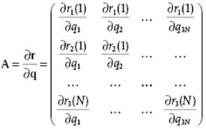
Note that the matrix A is orthogonal, that is, A⁻¹ = A^T. For the velocity we obtain

(2.48)

2.2.2 Hamilton's Principle and Lagrange's Equations

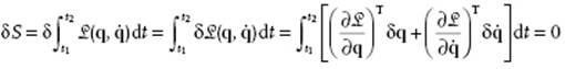
Almost always, the most economic description of physical laws is in the form of an extremum principle, and this is also the case with classical mechanics. Hamilton's principle [6, 7] states that, using a certain function called the Lagrange function (and to which we come in some detail later), the action S defined by

(2.49)

is minimal for the actual path of q(t) given q(t₁) and q(t₂) at times t₁ and t₂. The principle thus states that the motion of an arbitrary system occurs in such a way that the variation of the action δS vanishes provided that the initial and final states are prescribed. Since is a scalar, it is immaterial in which coordinate system it is expressed. In particular it may be expressed in generalized coordinates.

Evaluating Hamilton's principle using variation calculus (see Appendix B) results in

Partial integration of the 2nd term of the previous equation using yields

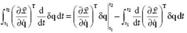
The boundary term vanishes since δq vanishes at the boundary. Combining results in

and, since the variations δq are arbitrary, we obtain for the equations of motion

(2.50)

These so-called Lagrange equations, given the Lagrange function , describe the behavior of a holonomic system. One can show that, using this description, is defined to within an additive total time derivative of any function of the coordinates.

A basic assumption of nonrelativistic classical mechanics is that space-time is isotropic and homogeneous, that is, a so-called inertial frame can be found in which the laws of mechanics do not depend on the position and orientation of the system in space and are independent of the time origin. From the requirement that the behavior of a free particle is the same in any coordinate system moving with constant velocity, it follows that or , representing the kinetic energy, and where v is the velocity of the particle with respect to the inertial frame and the proportionality factor m is the mass. For a set of free particles the Lagrange function represents the total kinetic energy T so that , where the mass matrix M′ is defined by

(2.51)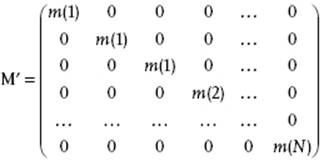

Consider now a system of particles that interact with each other but not with other bodies, described by a potential energy function which we take as −Φ(r) so that becomes . Using as generalized coordinates Cartesian coordinates, substitution in the Lagrange equations results in m_idv_i/dt = −∂Φ/∂r_i ≡ f_i representing Newton's Second Law. From this law, alternatively written as d(mv)/dt = f = −∂Φ/∂r, we infer Newton's First Law, v = constant if f = 0. The force f = −∇Φ(r) depends only on the coordinates r. It is called conservative because the work done by f, when moving a particle from one point to another, is independent of the path taken.

Transforming to generalized coordinates, the kinetic energy T can be expressed as

(2.52)

with M = A^TM′A the generalized mass matrix. In general therefore, T must be considered as a function of q and , that is, . We write for the set of forces f(i), as before, f^T = [f₁(1),f₂(1),f₃(1),f₁(2), … , f₃(N)]. If the force f is conservative, that is, if f = −(∂Φ/∂r), the generalized force Q is conservative as well and given by

(2.53)

Using the Lagrange function and realizing that , we may write

(2.54)

which are the Lagrange equations of motion for a conservative system describing a system of N particles with 3N second-order equations.

Example 2.3: The harmonic oscillator

For a harmonic oscillator the kinetic energy T is given by T = ½mv², while the potential energy Φ is described by Φ = ½kx². Here, m is the mass, v = dx/dt is the velocity, k is the force constant, and x is the position coordinate of the particle. For the generalized coordinates we thus take the Cartesian coordinates and the Lagrange function reads . From the Lagrange equations , we have

Combining yields . Solving this differential equation leads to x = x₀exp(iωt) with ω = (k/m)^1/2 and x₀ the amplitude. Equivalently x = x₀cos(ωt + φ₀), where φ₀ is the phase.

Problem 2.10*

Show that for a free particle the Lagrange function with v the velocity of the particle. Also show that in an inertial frame a free particle will move with constant v. Finally, show that the mass m > 0.

Problem 2.11*

Show that the Lagrange function is defined to within an additive total time derivative of any function of the coordinates.

2.2.3 Conservation Laws

In principle, there exist 3N−1 functions of q and , called integrals (or constants) of the motion, whose values remain constant during the motion. The most important of these are derived from the isotropy and homogeneity of space and time.

Let us consider homogeneity of time. Due to this homogeneity, the Lagrange function of a closed system is explicitly independent of time. Hence,

(2.55)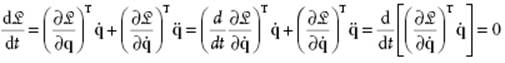

where in the 2nd step the Lagrange equations are used. So we obtain

(2.56)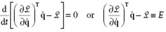

We thus have as one integral of the motion the energy E of the system. This relation is also valid for systems in a constant external field since in that case is still valid. If with T a quadratic function of , Euler's theorem for homogenous functions results in

(2.57)

Consequently, the constant of the motion energy E equals the sum of T and Φ.

Let us now consider homogeneity of space and use an infinitesimal displacement dε. For a parallel displacement, where every particle is moved by the same amount dε, the variation in should be zero and is given by

(2.58)

Because dε is arbitrary we have and using the Lagrange equations results in

(2.59)

Hence, changing to direct notation, for a closed system the momentum vector is conserved during the motion. It will be clear that p is additive over the individual particles i, independent of whether interaction is present or not. The interpretation follows from the expression which determines the force on particle 1. Since , the total force f = Σ_if_i is zero. In particular, for two particles f₁ + f₂ = 0 , where f₁ denotes the force exerted on particle 1 by particle 2. This represents Newton's Third Law implying that the force by particle 1 exerted on particle 2 is equal to, but is oppositely directed, to the force exerted by particle 2 on particle 1, both lying along the line joining the particles. From this result one can show that the total energy E is given by E = ½μV² + E_int with total mass μ = Σ_im_i and V = p/μ the velocity of the center of mass, the latter being given by R = Σ_im_ir_i/μ and E_int the energy of the system being at rest as a whole (see Problem 2.13). The same result follows if is given in generalized coordinates q, in which case p_i and f_i are denoted as the generalized momenta and generalized forces, respectively.

Let us finally consider isotropy of space and use an infinitesimal angle of rotation dϕ around a vector ϕ. The variation in radius vector r for any particle is δr = dϕ × r, while the variation in velocity v reads δv = dϕ × v. For a rotation where each particle is rotated by the same amount dϕ, the variation in should be zero and in direct notation¹⁴⁾ reads

(2.60)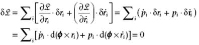

or, taking dϕ outside after permutation of factors,

(2.61)

Because dϕ is arbitrary, we have dΣ_i(r_i × p_i)/dt = 0, and therefore for a closed system the angular momentum vector l ≡ Σ_ir_i × p_i is conserved during the motion. Like the momentum vector p, it is additive over the particles of the system.

For a collection of connected particles, three types of forces can be distinguished. First, forces acting alike on all particles due to long-range external influences. Examples of this type of force are the gravity force or forces due to externally imposed electromagnetic fields. We call them volume (or body) forces and indicate them again for a particle i by f_vol(i). Second, forces applied to a particle due to short-range external forces. Examples of this type are interactions with walls of an enclosure. We call them surface (or contact) forces and indicate them by f_sur(i). Volume and surface forces are collectively called external forces, f_ext(i), that is, f_ext(i) = f_vol(i) + f_sur(i). Third, forces due to the presence of the other particles, that is, internal loading. These internal forces are indicated by f_int(i). Let f_pp(ij) denote the force on particle i due to particle–particle interaction with particle j. Then according to Newton's Third Law we have

(2.62)

The resultant internal force acting on particle i is then

(2.63)

and the total force on particle i is

(2.64)

Returning to the subscript notation, the system of particles is in equilibrium if the force f_i on each particle i in the system is equal to its rate of change of linear momentum dp_i/dt, also known as the inertial force. Obviously, we have

Motions of the collection of all particles that leave the distances between particles unchanged are called rigid body motions. Clearly, according to Newton's Third Law, the work due to internal forces vanishes for rigid body motion.

Example 2.4: The harmonic oscillator again

In a harmonic oscillator an external force f acts on a mass m and is linearly related to the extension x, that is, f = −kx, where k is the spring constant. The force f can be obtained from the potential energy Φ = ½kx² via f = −∂Φ/∂x. If the momentum and velocity are given by p = mv and v, respectively, Newton's Second Law reads . Combining leads to . Defining the circular frequency ω = (k/m)^1/2, the solution of this differential equation is x = x₀exp(−iωt), as in Example 2.3.

Problem 2.12

An object of mass m moves in a plane with speed v at a constant distance r to the center of rotation. Let x be the position of the object in the plane with the origin as the center of rotation. Show that:

a) the angular speed ω = v/r and acceleration ,

b) the angular momentum l = mvr = Iω with I = mr² the moment of inertia,

c) the torque , and

d) the kinetic energy T = ½Iω² = l²/2I.

Problem 2.13

Show that the total energy E of a system of particles is given by E = ½μV² + E_int with total mass μ = Σ_im_i, V = p/μ the velocity of the center of mass (given by R = Σ_im_ir_i/μ) and E_int the energy of the system being at rest as a whole.

2.2.4 Hamilton's Equations

The above formalism may be put in more convenient form by introducing the generalized momentum p defined by

(2.65)

Defining the Hamilton function by the Legendre transform (see Appendix B)

we obtain for its differential

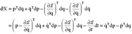
where in the last step use is made of Eqs (2.65) and (2.50). For the equations of motion we thus obtain

(2.66)

which are known as Hamilton's equations of motion and, because of their symmetry and simplicity, also are often called the canonical equations of motion. In this way the system is described by 6N first-order equations instead of the 3N second-order equations. The motion of set of particles can thus be described by a trajectory in a 6N-dimensional space, the so-called phase space, with coordinates q and p. The phase space is an essential concept in statistical mechanics.

Formally, for a change of the Hamilton function with time t, we have

Using Hamilton's equations it is easy to show that the first two terms cancel so that

(2.67)

Thus, a Hamilton function explicitly independent on time (but only implicitly via p and q) is constant, that is, where E is that constant. To interpret this constant for systems described by a Lagrange function , we consider and obtain

(2.68)

This result shows that the constant E equals the already defined energy but now expressed in terms of position and momentum as independent coordinates. As noted before, for a system with a time-independent potential, the energy and thus the Hamilton function is explicitly independent of time and the system is conservative. Finally, since is a function of q and p, we must express T also in terms of p. Inverting , we obtain . Hence

(2.69)

The Hamilton function thus reads . Note that the generalized force Q = A^Tf is not equal to . This is only true if M is independent of q, which generally is not the case.

Example 2.5: The harmonic oscillator once more

We treat once more the oscillator with kinetic energy T = ½mv² = p²/2m and potential energy Φ = ½kx². From Hamilton's equation , we get right away , resulting in the solution indicated in Example 2.3. From Hamilton's we have the identity .

Problem 2.14

Verify Eqs (2.66) and (2.67).

Problem 2.15

Show that for a conservative system using .