Liquid-State Physical Chemistry: Fundamentals, Modeling, and Applications (2013)

14.3. Solvent Effects

The description of reactions given in Section 14.2 is for gas-phase reactions. Although the study of gas-phase reactions has led to a great deal of insight into reaction mechanisms, in practice most reactions are carried out in liquids. The difference between a gas-phase reaction and a liquid-phase reaction is related to the presence of a solvent. In solution reactants are usually solvated, that is, bound to one or more solvent molecules. The transport of reactants in liquids, depending on the diffusion coefficients, is more hampered then in gases; moreover, the solvent may catalyze the reaction and thus change the mechanism. The reaction rate will thus be influenced not only by temperature and concentrations but also by the type of solvent. Whereas, reactions involving ions are rare in gas-phase reactions, they are abundant in liquid-phase reactions. Therefore, electrostatic forces, dependent on permittivity and ionic strength, are also important. Finally, pressure will influence the rate of reaction. Before discussing these effects, we should briefly sketch the situation of a solute in a solvent and some associated preliminaries. We note upfront that the analysis is a mixture of molecular and macroscopic arguments in which macroscopic physical properties of solvents are used.

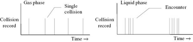
In the discussion of simple liquids in Chapter 8, we indicated that there is only some justification for the lattice model in which a molecule occupies for a certain time a cell formed by its neighbors. Such a cell exists only for about 10 collisions. However, in molecular solutions the cell for a solute, in this connection denoted as cage, exists somewhat longer. Indeed, in time, two reactants will meet in the same cage and collide many times, perhaps 20 to 200 times [6], before they either diffuse further or react in that period. Such a set of events is called an encounter. The time between encounters is large when compared to the time between collisions within an encounter. In the gas phase, the time interval between collisions of reactants is much more homogeneously distributed (Figure 14.2). With respect to reactions, the lower frequency of encounters is compensated by the higher frequency within an encounter, as evidenced by the near constancy of rate constants for certain reactions.

Figure 14.2 Collision pattern between reactants in the gas phase and in the liquid phase.

There is some experimental evidence for the cage effect from, for example, the photochemical decomposition [8] of CH₃NNCH₃ and CD₃NNCD₃. The absorbed light dissociates the molecules in N₂ molecules and CH₃ and CD₃radicals. In the gas phase the latter recombine to ethane in proportions that indicate a random mixing before recombination, whereas in i-octane only C₂H₆ and C₂D₆ are formed. This absence of CH₃CD₃ indicates that the radicals are kept together by the cage until recombination occurs.

With this cage model in mind, we can distinguish three stages for a reaction: 1) the diffusion of reactants A and B towards each other to form the encounter pair (A···B) in a cage; 2) the reaction of the reactants (A···B) in the cage to products (X···Y); and 3) the separation of products (X···Y) away from each other. These processes can be represented by

(14.25)

The rate of reaction, as measured by d[A]/dt, is given by

(14.26)

while the rate of formation of the encounter pair (A···B) is given by

(14.27)

Now, we assume steady-state conditions for (A···B), that is, d[(A···B)]/dt = 0, so that

(14.28)

Substitution of Eq. (14.28) in Eq. (14.26) results in

(14.29)

There are two limiting conditions. First, for k_R << k_−D, k ≅ k_R(k_D/k_−D) and the rate becomes

(14.30)

In this case we have reaction control. Second, for k_R >> k_−D, k ≅ k_D and the rate becomes

(14.31)

and we have diffusion control. The behavior for these limiting behaviors is discussed in the next two sections.

We limit the discussion to the physical effects of solvents, where the pro­perties of the solvents influence the rate but the solvent does not participate as a reactant. For these aspects we refer to, for example, Buncel et al. [7] and Reichardt [8].

Problem 14.2

Verify Eq. (14.29) to (14.31).