Liquid-State Physical Chemistry: Fundamentals, Modeling, and Applications (2013)

14.7. Ionic Solutions

In Chapter 11 we derived the activity coefficients for ionic solutions using the Debye–Hückel theory, which can be used immediately if the structure of the activated complex is known. For this structure, two extremes have been proposed: (i) a double-sphere model; and (ii) a single-sphere model. Each of these models will be discussed in the following sections (Figure 14.5).

Figure 14.5 The double-sphere and single-sphere models for the activated complex in an ionic reaction.

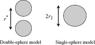
14.7.1 The Double-Sphere Model

For the double-sphere model consider the reaction A + B → M^‡, where the reactants have charges z_Ae, z_Be and (z_A + z_B)e, respectively. The activated complex is considered to be a double-sphere with r* the distance between A and B. The concentration of the activated complex is taken as proportional to the bulk concentration of A multiplied by the average concentration of B at a distance r*. The latter is given by

(14.57)

where c_B is the bulk concentration of B, ψ is the mean electrostatic potential at a distance r* from A, and e is the unit charge. Hence, the concentration of activated complex is

(14.58)

with k′ the proportionality constant. Using the Debye–Hückel expression for ψ (Eq. 12.48), the expression becomes

(14.59)

where a is the mean distance of closest approach of A and B. The parameter κ is defined by the Debye length κ² = 2N_Ae²I_c/ε₀ε_rkT, where N_A is Avogadro's constant and the ionic strength I_c is defined by . At high dilution, Eq. (14.59) becomes

(14.60)

and since the activity coefficient γ is equal to c⁰/c, we obtain

(14.61)

or, using Eq. (14.59) and (14.60)

(14.62)

The activity coefficient is with reference to the infinitely diluted solution, but we need this with respect to the gas phase. Here, we use α for the activity coefficient of the solution with respect to the gas phase, β for the activity coefficient of an infinitely diluted solution with respect to the gas phase, and γ for the activity coefficient of the solution with respect to the infinitely diluted solution. So

(14.63)

where the quantity involving the β-terms is given by

(14.64)

and the subscript “gas” indicates the ideal gas state with permittivity ε_r = 1. Applying the Debye–Hückel expression, this reads

(14.65)

Eliminating the activity coefficients α using Eq. (14.62), (14.63) and (14.65), the final result for the double-sphere model employing k_AB = k_AB,0(α_Aα_B/α_‡) is

(14.66)

14.7.2 The Single-Sphere Model

For the single-sphere model, one uses essentially the Born hydration model (see Section 12.2). The activated complex is considered to be a single-sphere of radius r, which is transferred from the gas phase to the liquid phase. For this process we showed in Chapter 12 that

(14.67)

and because for this process ΔG = kT lnβ (with β as the activity coefficient defined in the previous section), we obtain

(14.68)

Hence, it follows that

(14.69)

where r_‡ is the radius of the (spherical) activated complex with charge (z_A + z_B)e. The activity coefficient γ is as given by the Debye–Hückel model (see Section 12.5)

(14.70)

and, if a mean distance a is assumed for the distance of closest approach of the ions, it follows that

(14.71)

Now, employing again k_AB = k_AB,0(α_Aα_B/α_‡) and introducing Eq. (14.69) and (14.71) in the α-terms of Eq. (14.63), the final result becomes

(14.72)

The expressions for the single-sphere and double-sphere models become identical when r_A = r_B = r_‡. The expressions derived in this and the previous section can be tested in two ways: first, via the dependence on ionic strength while keeping the permittivity constant; and, second, via the dependence on permittivity of the solvent using data for infinite dilution, that is, extrapolated to zero ionic strength. This will be discussed in the next two sections.

Problem 14.4

Verify Eq. (14.66) and (14.72).

Problem 14.5

Discuss the difference in dependence on ionic radii between the single-sphere and double-sphere models for the rate constant. To that purpose, express r_A, r_B and r_‡ for the single-sphere model in r*, and consider when the resulting expression differs significantly from the corresponding expression for the double-sphere model. Do you expect that experimental data on the rate constant can help to distinguish between the two models?

14.7.3 Influence of Ionic Strength

For both Eq. (14.66) and (14.72) the influence of the ionic strength is given by

(14.73)

where is the rate constant for infinite dilution. Inserting = 2e²N_AI_c/εkT (Eq. 12.48) and neglecting κa in the term 1 + κa in comparison with unity, this expression reduces to

(14.74)

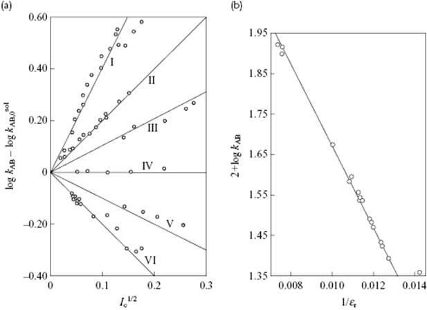
Introducing all numerical factors it appears that A = 1.02 (using mol l⁻¹ for molarity) for aqueous solutions at 25 °C. In a plot of k_AB versus , one should thus find a straight line with slope 1.02z_Az_B. The influence of the ionic strength for various reactions is shown in Figure 14.6a, where the experimental slopes nicely match the expected 1.02z_Az_B, including the zero slope if either z_A or z_B is zero.

Figure 14.6 Dependence of the specific rate constants on (a) ionic strength I_c and (b) permittivity ε_r. Panel (a): I. Co(NH₃)₅Br²⁺ + Hg²⁺, z_Az_B = +4; II. , z_Az_B = +2; III. , z_Az_B = +1; IV. CH₃CO₂C₂H₅ + OH⁻, z_Az_B = 0; V. H₂O₂ + H⁺ + Br⁻, z_Az_B = −1; VI. Co(NH₃)₅Br²⁺ + OH⁻, z_Az_B = −2. Panel (b): The reaction between bromoacetate and thiosulfate in various media. Data from Ref. [11].

Of course, deviations occur when the solution is too concentrated, that is, if I_c is too high. This occurs first, due to the further (mathematical) approximation made in the Debye–Hückel expression and, second, due to the approximate nature of the Debye–Hückel model itself. Moreover, for solvents with a low permittivity, the association of the ions may cause discrepancies, as has been shown for the reaction of sodium bromoacetate (Na⁺BrAc⁻) with sodium thiosulfate . At high dilutions BrAc⁻ reacts with so that z_Az_B = +2. However, at higher concentrations the complexes Na⁺···BrAc⁻, and are formed, and the effective value of z_Az_Bchanges to zero. The repulsion between the negatively charged ions BrAc⁻ and is decreased by the formation of complex ions, such that the specific reaction rate increases.

14.7.4 Influence of Permittivity

For a solution with ionic strength equal to zero, the terms in in Eq. (14.66) and (14.72) disappear and we are left with only the effect of the permittivity. Plotting lnk_AB, extrapolated to zero ionic strength, versus 1/ε_r results for Eq. (14.66) in

(14.75)

while for Eq. (14.72) one obtains

(14.76)

Both expressions give the same order of magnitude answer because the values of r*, r_A, r_B and r_‡ are not too different. From Eq. (14.75) it is immediately clear that the slope has a negative sign if the ions are similarly charged, and positive if they are oppositely charged. This result can also be obtained from Eq. (14.76).

The influence of the permittivity on the rate constants extrapolated to zero ionic strength for the reaction between bromoacetate and thiosulfate in various media is shown in Figure 14.6b. Here, the line corresponds to a value of r* = 0.51 nm, but a good fit can also be obtained by using r_A = 0.33 nm (bromoacetate), r_B = 0.17 nm (thiosulfate) and r_‡ = 0.50 nm (activated complex), respectively. The use of mole fractions instead of volume fractions (which are actually used in the single-sphere model) leads also to a good fit with r* = 0.56 nm. Yet, deviations can also occur, in particular for low-permittivity solvents.

Problem 14.6: The dissociation of AgNO₃

The dissociation constants K for AgNO₃ in H₂O and C₂H₅OH are 1170 × 10³ mol l⁻¹ and 4.42 × 10³ mol l⁻¹, respectively. Estimate the value for K in CH₃OH using the double-sphere model, and compare the result with the experimental value K = 20.5 × 10³ mol l⁻¹. Estimate the value for 2r* and compare the result with the sum of the Stokes radii for Ag⁺ and . Use, where necessary, data from Appendix E.