Liquid-State Physical Chemistry: Fundamentals, Modeling, and Applications (2013)

In Chapter 2 we reviewed general thermodynamics but avoided phase transitions. In this chapter, we discuss some aspects of these phenomena, dealing first with some general aspects and thereafter with discontinuous and continuous transitions, in particular the latter providing a rich part of physical chemistry.

16.1. Some General Considerations

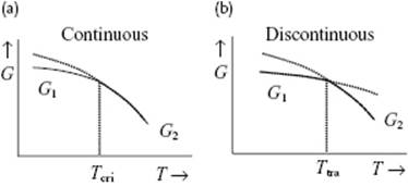
By changing the conditions – such as P or T – for many materials, a transition from one phase to another can be induced. Under certain conditions even two phases of the same material may coexist. As each of the two phases has its own Gibbs energy expression, under these conditions the chemical potentials of the phases are equal. The Gibbs energy G itself is always continuous over the transition, but the partial derivatives ∂G/∂T and ∂G/∂P may be discontinuous (Figure 16.1). In that case, the phase transformation is denoted discontinuous¹⁾ (or first-order), while for the situation where the first derivative is continuous, but the higher derivatives are either zero or infinite, one speaks of a continuous (or second-order) phase transition.

Figure 16.1 Schematic of the behavior of the Gibbs energy G for two phases around (a) continuous phase transition and (b) discontinuous phase transformation. In both cases the stable states below the transition temperature have a Gibbs energy G₁, while above the transition temperature the Gibbs energy is G₂. The continuous transition occurs at the critical temperature T_cri with a continuous change in G, that is, ∂ΔG/∂T = 0, where ΔG = G₂ − G₁. The dotted line indicates the metastable continuation of the high temperature G below T_cri. The discontinuous transition occurs at a certain transition temperature T_tra with a discontinuous change in G (∂ΔG/∂T ≠ 0).

The angle of intersection of the G₁ and G₂ curve for phases 1 and 2, respectively, determines the entropy and volume change associated with the phase transformations, and hence the type of phase transition. Experimentally, it appears that by moving along the liquid–vapor (L-V) coexistence line over the critical point (CP), the differences in properties, in particular the density, between the liquid and gas phase vanish in a continuous way and the transition is continuous (Figure 16.2). Moving across the L-V curve from the liquid to the gas phase, and vice versa, leads to a discontinuous transition.

Figure 16.2 (a) Schematic of the phase equilibrium between the solid (S), liquid (L), and vapor (V) phase in the P–T plane, showing the triple point (TP) and critical point (CP). These are natural reference points as the melting temperature T_m and boiling temperature T_b depend on the environment, in particular the pressure P. For water, for example, P_cri = 218.3 atm, T_cri = 374.15 °C, ρ_cri = 320 kg m⁻³, and T_tri = 0.01 °C. While the transition over a coexistence line relates to a discontinuous phase transition, the transition over the critical point along the coexistence line relates to a continuous phase transition; (b) Schematic of the phase equilibrium in the P–V plane. The horizontal line indicates the equal area Maxwell construction. Above the CP only gases (G) can exist. The binodal line indicates the demarcation of global stability, while the spinodal line indicates the limits of local stability.

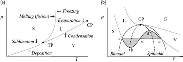
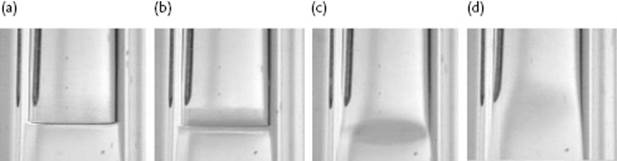
Following the coexistence (vapor pressure) line between liquid and vapor in the P–T diagram, we end at the critical point with temperature T_cri. In this process the density of the liquid decreases, while the density of the gas increases. At T_cri, the gas density ρ_gas and liquid density ρ_liq become identical. Moreover, for T < T_cri a meniscus – that is, a sharp transition region between liquid and vapor – is present except for temperatures close to T_cri (say within one degree), where the meniscus widens and suddenly disappears at T_cri. Figure 16.3 illustrates this behavior²⁾.

Figure 16.3 The disappearing of the meniscus of benzene along the coexistence curve from far below (a) to close to (b) and just below (c) to just above T_cri (d).

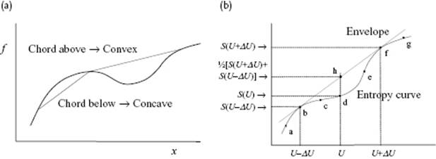
Before discussing some ideas on how to describe transitions, let us first discuss some stability considerations. For this we need the concept of convexity. A curve is convex (or convex up) if the chord is above the curve, whereas a curve is concave (or convex down) is the chord is below the curve (Figure 16.4a). Thermodynamics requires that for changes in entropy we always have (ΔS)_U ≥ 0, which implies that entropy S is concave over its entire domain. If we obtain from a model or from experimental data a curve such as abcdefg in Figure 16.4b, the above implies that the envelope abhfg must be considered as the acting entropy function. Considering for the moment S as function energy U and volume V, concavity of S results in

(16.1)

where the reduction to the differential form only follows if ΔU → 0. Similarly,

(16.2)

where again the differential form only follows if ΔV → 0. In fact, these considerations also apply for a combined change of U and V,

(16.3)

leading again to Eq. (16.1) and (16.2) as well as to (Problem 16.3)

(16.4)

Figure 16.4 (a) Concave and convex interval of a function; (b) The relation to stability. If the curve abcdefg represents the entropy S, say as obtained from a model, as a function of energy U, the curve abhfg represents the entropy to be used since the entropy curve should be always concave. The range bcdef represents global instability (binodal), while the range cde (with c and e inflection points) represents local instability (spinodal).

So, the concavity leads to conditions for global stability while the differential forms lead to conditions for local stability. For example, Eq. (16.1) leads to

(16.5)

indicating that the molar heat capacity C_V must be positive for a system to be thermally stable. Although Eq. (16.2) and (16.4) can also be used to establish further stability requirements, it is easier to employ thermodynamic potentials instead of the entropy. To that purpose, we first recall that the principle (ΔS)_U ≥ 0 is always equivalent to (ΔU)_S ≤ 0, stating that the energy U should always be convex. This leads to

(16.6)

(16.7)

which is fully analogous to the entropy case. It is convenient to consider also the Helmholtz and Gibbs energy. We first note that, if we have U(S,V) and F(T,V), then T = ∂U/∂S and S = −∂F/∂T, respectively. Therefore

(16.8)

Hence, the sign of ∂²F/∂T² is the negative of the sign of ∂²U/∂S², implying that if U is a convex function of S, then F is a concave function of T. This type of result holds for all transforms, so that we obtain for the Helmholtz function and Gibbs function, respectively,

(16.9)

Summarizing, the thermodynamic potentials – that is, the energy and its Legendre transforms – are convex functions of their extensive variables and concave functions of their intensive variables³⁾.

From Eq. (16.9) we easily obtain

(16.10)

indicating that the isothermal compressibility κ_T must be positive for a system to be mechanically stable⁴⁾. By combining C_V ≥ 0 and κ_T ≥ 0 with κ_T − κ_S = TVα²/C_P and C_P − C_V = TVα²/κ_T (see Chapter 2, Eq. 2.28), one can further infer that

(16.11)

The first of these equations states that, upon the addition of heat to a system, the temperature rises but more at constant volume than at constant pressure. The second equation states that, upon decreasing the volume of the system, the pressure increases, but more at constant temperature than at constant entropy.

Problem 16.1

Near the critical point the density profile of molecules with molar mass M over the meniscus is significantly influenced by gravity. If we describe the gravitational potential (approximately) by ϕ = gh, with g the acceleration due to gravity and h the height, the equilibrium condition reads d(μ + Mϕ) = 0.

a) What is the expression for the molar volume V_m?

b) Calculate the pressure P at height h with respect to the meniscus level h₀.

c) Calculate the density ρ = M/V_m as a function of height h with respect to h₀.

d) In many cases properties are scaled with respect to their value at critical point, for example, T_red = T/T_cri, P_red = P/P_cri and V_red = V/V_cri. What is the appropriate expression for μ_red in terms of P_cri, V_cri and T_cri?

e) Scaling the equilibrium condition d(μ + Mϕ) = d(μ + Mgh) = 0, we obtain dμ_red = −dh_red. Calculate h_cri in h_red = h/h_cri.

f) Consider Ne and H₂O. For which compound is the width of the transition zone between liquid and gas near the critical point as characterized by h_cri larger? What does the order of magnitude of h_cri indicate to you? Use data as given in Appendix E.

Problem 16.2

Using the relation ∂²U/∂V² ≥ 0, show that κ_S ≥ 0.

Problem 16.3

Show by expanding the left-hand side of Eq. (16.3) in a Taylor series to second order that:

where S_UU ≡ ∂²S/∂U², S_UV ≡ ∂²S/∂U∂V, and S_VV ≡ ∂²S/∂V². Recalling that S_UU ≤ 0, show that this expression can be written as

and that this subsequently leads to Eq. (16.4).