Liquid-State Physical Chemistry: Fundamentals, Modeling, and Applications (2013)
16. Some Special Topics: Phase Transitions
16.3. Continuous Transitions and the Critical Point
For continuous phase transitions, considerable effort has been paid to adequately describe and understand the process, and this has led to an image that captures the essentials well. We recall that thermodynamic equilibrium is determined by minimization of the appropriate potential with respect to the internal variable or variables. Because η = Δρ = ρ − ρcri is single-valued above Tcri and has two values below Tcri, this difference is conventionally used as the internal variable (see Chapter 2) characterizing the liquid–gas transition. In connection with transitions, the internal variable used is normally called the order parameter. In the sequel of this section we first discuss some experimental facts, and thereafter mean field theory.
16.3.1 Limiting Behavior
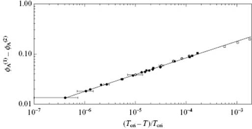
Both, single compounds and mixtures exhibit continuous transitions. In Figure 16.6 the relative density (ρL − ρV)/2ρcri of CO2 versus the relative temperature t ≡ (T − Tcri)/Tcri is given, while Figure 16.7 shows the difference in volume fraction (ϕ(1) − ϕ(2)) for CCl4 in C7F14 versus t. In both cases, the behavior is described by a power law [3].
Figure 16.6 The relative density (ρL − ρG)/2ρcri of CO2 versus the relative temperature −t = (Tcri − T)/Tcri with Tcri = 304.18 K, as described by (ρL − ρG)/2ρcri = B(−t)β with B = 1.85 and β = 0.340 ± 0.015.
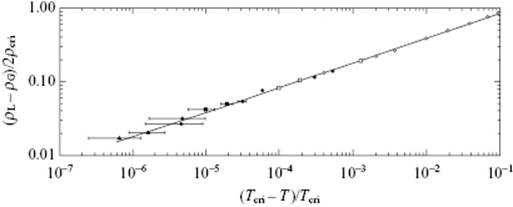
Figure 16.7 The difference in volume fraction ϕ(1) in the upper phase and ϕ(2) in the lower phase for CCl4 in C7F14 versus the relative temperature −t = (Tcri − T)/Tcri with Tcri = 301.786 K, as described by ϕ(1) − ϕ(2) = B(−t)β with B = 1.81 and β = 0.335 ± 0.020.
This type of experiment has led to the definition of various critical exponents. A critical exponent of a function, say a for a function f(x) of x, is defined by
(16.25) ![]()
and we write f(x) ∼ xa. This does not imply that f(x) = Axa, but rather that f(x) = Axa(1 + Bxb + …) with b > 0, and where Axa is called the singular part of f(x) and (1 + Bxb + …) the regular part or background function. The exponent7) a defines the rate of approach of f(x) to zero for a > 0 or to infinity for a < 0. If a = 0, the result is ambiguous. In this case f(x) has either a discontinuity or else a logarithmic singularity, that is, f(x) behaves like ln(T − Tcri).
The order parameter, that is, Δρ along the saturation curve for T < Tcri, is described by
(16.26) ![]()
where B and β are parameters and (1 + …) is the background function to which the critical exponent β is insensitive. Experimentally, the range for β is 0.3 < β < 0.4.
The response function – that is, the compressibility κT – behaves similarly but becomes infinite at T = Tcri. For T < Tcri (for ρ = ρliq or ρ = ρgas on the saturation curve) and T > Tcri (for ρ = ρcri), κT is described by, respectively,
(16.27) ![]()
where C, C′, γ, and γ′, are parameters and ![]() is the compressibility of an ideal gas with molecules of mass m at of density ρcri at Tcri. Experimentally, the range for γ and γ′ is 1.2 < γ < 1.4.
is the compressibility of an ideal gas with molecules of mass m at of density ρcri at Tcri. Experimentally, the range for γ and γ′ is 1.2 < γ < 1.4.
Such a power-law relation also holds for the heat capacity CV. This is given in a two-phase system for T < Tcri (for ρliq + ρgas = 2ρcri) and T > Tcri (for ρ = ρcri) by, respectively,
(16.28) ![]()
where A, A′, α and α′ are parameters. Experimentally, the range for α and α′ is −0.2 < α < 0.2.
For the pressure P along the critical isotherm T = Tcri, data are described by
(16.29) ![]()
where sgn(I) = 1 if I > 0 and sgn(I) = −1 if I < 0. Experimentally, we have 4 < δ < 5.
Finally, we examine the (total) pair correlation function h(r) = g(2)(r) − 1 (see Section 7.2). For large r, h → 0 and we expect, and also from Ornstein–Zernike theory it appears, that h(r) for T > Tcri behaves like
(16.30) ![]()
where f(r) is a weakly varying function8) of r, D is the dimension of space, and where the coherence (or correlation) length ξ measures the range of order in the liquid. In essence, ξ is a measure of the greatest distance from a given particle at which this particle can still cause nonrandom effects on the particle density. Under normal conditions the order of magnitude for ξ is a few molecular diameters, but for T → Tcri and ρ = ρcri, the value of ξ diverges to macroscopic size. In this case, high- and low-density regions appear on an increasingly larger scale until macroscopic regions of different density in the fluid lead to the two-phase region for T ≤ Tcri. However, the small(er) scale fluctuations do not disappear and within high-density regions there will be smaller regions of lower density, and vice versa. As soon as ξ approaches the wavelength of visible light, say 0.5–0.8 μm, these fluctuations lead to the phenomenon of critical opalescence. Using experimental data it appears that ξ also scales with T and for T < Tcri (for ρ = ρliq or ρ = ρgas on the saturation curve) and T > Tcri (for ρ = ρcri) is given by, respectively,
(16.31) ![]()
Using the result from Eq. (16.30), Fisher [4] showed that for D = 2, h(r) ∼ lnr, that is, increases with increasing r, which is physically impossible. He therefore introduced the additional exponent η (obeying 0 < η < 2) for r → ∞ at (ρ = ρcri) and (ρ = ρcri and T = Tcri), respectively, by
(16.32) ![]()
It appears that in 3D the value of η is small, typically about 0.03. Moreover, η is related to ν and γ (Example 16.1).
Example 16.1: The Fisher relation
In Chapter 6 we derived for the compressibility
![]()
Using h(r) → HDexp(−r/ξ)/rD−2+η we obtain
![]()
with x = r/ξ. If η < 1, the integral converges and it has value 1 for η = 0. Because κT ∼ t−γ, ![]() and ξ ∼ t−ν, we have
and ξ ∼ t−ν, we have
![]()
There appear to be more relations between the critical exponents. They were originally derived as (thermodynamic) inequalities between the various critical exponents, and usually named after their discoverer. We have for example,
(16.33) ![]()
(16.34) ![]()
(16.35) ![]()
Later, we will see that they actually are equalities and, moreover, that α′ = α and γ′ = γ. The derivation of some of them is easy, but for others it is quite involved. As an example we derive the Rushbrooke inequality. To do so we need Stanley's lemma that states that for f(x) ∼ xa and g(x) ∼ xb with f(x) ≤ g(x) and for 0 < x < 1, so that ln x < 0, we have a ≥ b. From thermodynamics, we know that CP − CV = TVα2/κT (all quantities positive, see Section 2.1), so that CP ≥ TVα2/κT. Because we have for the heat capacity CP ∼ (−t)−α′, for the compressibility κT ∼ (−t)−γ′, and for the thermal expansion coefficient α ∼ (−t)β−1, we obtain at once −α′ ≤ γ′ + 2(β − 1) or α′ + 2β + γ′ ≥ 2 (for 0 < α′ < 1, while for α′ ≤ 0, the most we can say is that 2β + γ′ ≥ 2).
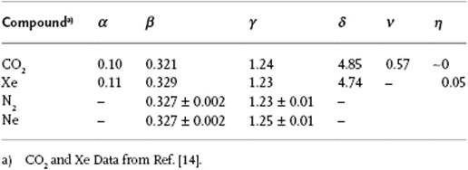
Furthermore, it appears that the critical exponents for a number of phenomena are essentially the same (Table 16.2). This happens to be the case if, for two phenomena, both the spatial dimensionality, for example, 2D or 3D, and the dimensionality of the order parameter, for example, a scalar or vector, are the same. These phenomena are said to belong to the same universality class. For the phenomena listed in Table 16.2 the lattice gas model (see Appendix C), with a scalar order parameter, forms the prototype. The liquid–gas transition also belongs to this class (Problem 16.9). We limit ourselves entirely to this class, and some experimental results are given in Table 16.3.
Table 16.2 Critical points and their order parameters.a)
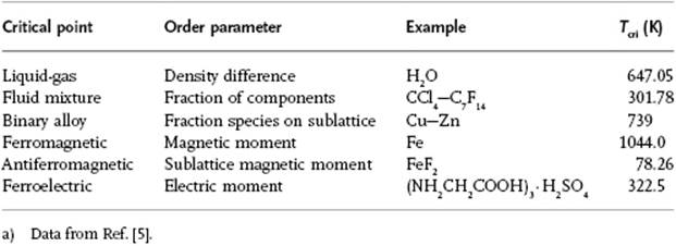
Table 16.3 Experimental values of critical exponents for various fluids.
16.3.2 Mean Field Theory: Continuous Transitions
Remember that in thermodynamics the equilibrium situation is conveniently obtained by minimizing the proper thermodynamic potential, say the “generalized” Helmholtz energy F(η;T,V), dependent on temperature T, volume Vwith respect to the order parameter (internal variable) η. We used the designation “generalized” because the “generalized” F only becomes the thermodynamic F after minimization with respect to η. In general, η varies with position, that is, is a field quantity, and we have to use the energy density. For a uniform distribution of η we can use the energy itself, but we will still use the energy density, here denoted by ![]() or by just
or by just ![]() or
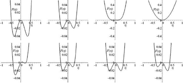
or ![]() . The order parameter η can be a local average of an underlying microscopic parameter describing the physics of the system. For example, for a ferromagnetic material the order parameter is the magnetization m which in the lattice model (see Appendix C) results as the average of the magnetic spins σ with value ±1. Above Tcri, m = 0, while below Tcri the magnetization is ±m. The order parameter η can also be purely macroscopic. For example, for a fluid the order parameter is conveniently taken as the density difference Δρ between liquid and gas. In Figure 16.8 the qualitative shape of the F(η;T,V) curves as a function of temperature for various conditions of V and T for a fluid are given. The simplest approach to describe these curves is to use the so-called mean field approach, originally due to Landau.
. The order parameter η can be a local average of an underlying microscopic parameter describing the physics of the system. For example, for a ferromagnetic material the order parameter is the magnetization m which in the lattice model (see Appendix C) results as the average of the magnetic spins σ with value ±1. Above Tcri, m = 0, while below Tcri the magnetization is ±m. The order parameter η can also be purely macroscopic. For example, for a fluid the order parameter is conveniently taken as the density difference Δρ between liquid and gas. In Figure 16.8 the qualitative shape of the F(η;T,V) curves as a function of temperature for various conditions of V and T for a fluid are given. The simplest approach to describe these curves is to use the so-called mean field approach, originally due to Landau.
Figure 16.8 The shape of the Helmholtz energy curve F. Upper row: Continuous transition along the coexistence curve where (from left to right) the images represent the shape changing to Tcri (mid-right) and above Tcri (outer-right); Lower row: Discontinuous transition across the coexistence curve where images (from left to right) represent the shape change from liquid via coexistence line (mid-right) to gas (outer-right).
In this approach, ![]() typically represents the grand potential density (see Chapter 2), and we assume that the Helmholtz part F (η) of
typically represents the grand potential density (see Chapter 2), and we assume that the Helmholtz part F (η) of ![]() near Tcri can be expanded in a power series in η, reading
near Tcri can be expanded in a power series in η, reading
(16.36) ![]()
The driving force h is the conjugate variable to the order parameter η. For a fluid the driving force is the chemical potential μ (with order parameter Δρ), while for a ferromagnetic material mentioned above it is the external magnetic field H (with order parameter m). In principle, all coefficients an depend on temperature T. The parameter a0 is a reference energy and can be omitted. Equilibrium requires that ![]() , and in the absence of an external driving force, this requires that a1 is absent. Further note that a4 should be > 0 if the system is to be stable. In cases the order parameter η can have only the two values ±η, as for the magnetization case, the third-order terms must also be absent because
, and in the absence of an external driving force, this requires that a1 is absent. Further note that a4 should be > 0 if the system is to be stable. In cases the order parameter η can have only the two values ±η, as for the magnetization case, the third-order terms must also be absent because ![]() should equal
should equal ![]() . For the fluid case this is obviously not the case if we use η = Δρ = (ρ − ρcri). Nevertheless, we assume this to be true for the moment, that is, we essentially discuss the magnetic problem, and come back later to the case a3 ≠ 0. For the moment we also consider the case when h = 0. So, we are left with
. For the fluid case this is obviously not the case if we use η = Δρ = (ρ − ρcri). Nevertheless, we assume this to be true for the moment, that is, we essentially discuss the magnetic problem, and come back later to the case a3 ≠ 0. For the moment we also consider the case when h = 0. So, we are left with ![]() . As usual, equilibrium is reached when
. As usual, equilibrium is reached when ![]() and the solutions are simply found to be
and the solutions are simply found to be
(16.37) ![]()
The coefficient a2 can be expanded with respect to temperature reading ![]() , where
, where ![]() (generally
(generally ![]() ). Since for T < Tcri, η should be non-zero for η arbitrarily close to Tcri, we must have a2,0 = 0 and hence a2 = a2,1ΔT. A similar expansion could be used for a4, but as this will lead to second-order temperature effects, we take a4 as a constant. This implies that for T < Tcri, the solution is η* = ±(−a2,1ΔT/2a4)1/2. To ease the notation slightly, we write
). Since for T < Tcri, η should be non-zero for η arbitrarily close to Tcri, we must have a2,0 = 0 and hence a2 = a2,1ΔT. A similar expansion could be used for a4, but as this will lead to second-order temperature effects, we take a4 as a constant. This implies that for T < Tcri, the solution is η* = ±(−a2,1ΔT/2a4)1/2. To ease the notation slightly, we write
(16.38) ![]()
with a and b as the parameters, t as before, and omitting the asterisk from now on.
We now calculate the critical exponents. For T < Tcri the solution is η = (−at/2b)1/2, so comparing with η ∼ (Tcri − T)β results in β = ½.
For T > Tcri, η = 0 and thus ![]() . For T < Tcri, η = (−at/2b)1/2 and thus
. For T < Tcri, η = (−at/2b)1/2 and thus ![]() . Because
. Because ![]() , we easily obtain
, we easily obtain
(16.39) ![]()
The heat capacity thus changes discontinuously at Tcri, which can be represented by taking the exponent α = 0.
To compute the other exponents we need to let h ≠ 0. Equilibrium is obtained from ![]() and, using
and, using ![]() , reads h = 2atη + 4bη3. On the critical isotherm t = 0 and therefore h ∼ η3 so that δ = 3.
, reads h = 2atη + 4bη3. On the critical isotherm t = 0 and therefore h ∼ η3 so that δ = 3.
The response function, the isothermal susceptibility XT in this case, is given by
(16.40) ![]()
where η(h) is a solution of h = 2atη + 4bη3. Since for T > Tcri we have η = 0, XT = (2at)−1. Similarly, for T < Tcri at h = 0, we have η2 = −at/b, XT = (−4at)−1, and thus γ = γ′ = 1. Note that XT(T < Tcri) = −½XT(T > Tcri) always in this model.
16.3.3 Mean Field Theory: Discontinuous Transitions
Let us consider briefly whether the Landau approach can be applied to discontinuous transitions. So far, we have used ![]() . We omitted a linear term because we required that η = 0 for T > Tcri, and a cubic term on the basis of symmetry. We now allow the cubic term so that we have
. We omitted a linear term because we required that η = 0 for T > Tcri, and a cubic term on the basis of symmetry. We now allow the cubic term so that we have
(16.41) ![]()
Considering only the case that h = 0, we obtain equilibrium from ![]() and the solutions are found to be
and the solutions are found to be
(16.42) ![]()
with c ≡ 3c′/8b. The solution for T < Tcri is acceptable (i.e., real) if c2 − 2at/b > 0, that is, for a temperature t < t* ≡ bc2/2a. Because t* > 0, the temperature T* > Tcri, the latter being the temperature where the coefficient of η2vanishes. Recall that for the continuous transition an acceptable solution becomes available only for t < 0 or T > Tcri. Figure 16.8 (lower row) shows a schematic of the behavior for the discontinuous transition. For t > t*, ![]() shows only one minimum. For t < t* a secondary minimum appears which at t = t1 is equal to the one at η = 0. For t < t1 this minimum becomes the global minimum and the value of η jumps discontinuously to a nonzero value, representing the discontinuous transition. Note that η(t1) is not arbitrarily small, as required by Landau theory. Generally – but not always – the presence of a cubic term in η will give rise to a discontinuous transition.
shows only one minimum. For t < t* a secondary minimum appears which at t = t1 is equal to the one at η = 0. For t < t1 this minimum becomes the global minimum and the value of η jumps discontinuously to a nonzero value, representing the discontinuous transition. Note that η(t1) is not arbitrarily small, as required by Landau theory. Generally – but not always – the presence of a cubic term in η will give rise to a discontinuous transition.
16.3.4 Mean Field Theory: Fluid Transitions
Let us now return to our case of the liquid–gas transition for which a1, a3 ≠ 0. In this case, ![]() reads (using the chemical potential μ as the proper driving force)
reads (using the chemical potential μ as the proper driving force)
(16.43) ![]()
For the general case a solution of Eq. (16.43) is rather difficult to obtain. For the fluid case, however, we apply a trick by writing η = η0 + Δη. If we do so we obtain
(16.44) ![]()
(16.45) ![]()
(16.46) ![]()
(16.47) ![]()
(16.48) ![]()
Each of the functions B(η0), … , E(η0) can be considered as a function of temperature, which we expand to first order in T. The function A(η0,μ) depends on η0 and μ, so that a first-order expansion in T and μ with respect to Tcriand μcri reads ![]() with ΔT = T − Tcri and Δμ = μ − μcri using the notation
with ΔT = T − Tcri and Δμ = μ − μcri using the notation ![]() . We can eliminate the linear and cubic terms in Δη by setting them equal to zero. First, solving the cubic term D(η0) for η0 leads to η0 = −a3/4a4 = −a3,1ΔT/4a4. Substitution in the linear term B(η0) results, to first order in ΔT, in
. We can eliminate the linear and cubic terms in Δη by setting them equal to zero. First, solving the cubic term D(η0) for η0 leads to η0 = −a3/4a4 = −a3,1ΔT/4a4. Substitution in the linear term B(η0) results, to first order in ΔT, in
(16.49) ![]()
where the last step can be made because ΔTη0 is of second order in ΔT. Since B(η0) = 0 requires Δμ = a1,1ΔT, we see that this condition is already satisfied. Therefore, along the line determined by η0 = −a3,1ΔT/4a4, the Landau function ![]() will read
will read
(16.50) ![]()
which has the same form as ![]() for the magnetic problem. The solution accordingly is also the same and reads for T < Tcri
for the magnetic problem. The solution accordingly is also the same and reads for T < Tcri
(16.51) ![]()
All critical exponents are thus also the same as before. The complete solution is obtained by superposing the Δη solution on the η0 behavior. To interpret η0 we recall that η = η0 + Δη = ρ − ρcri. Using ηliq = η0 + Δη and ηgas = η0 − Δη, we see that ρliq + ρgas = 2η0, so that η0 equals the average density and represents the law of rectilinear diameters (see Chapter 4). Because η0 = −a2,1ΔT/4a4, the average density is a linear function of temperature, as approximately confirmed by experimental evidence. However, expanding all functions to second order leads to nonlinear behavior [6].
In conclusion to this part, we note that the order of magnitude of the critical exponents as obtained from the mean field approach is correct, but that quantitative agreement is missing. The Landau expression is approximate and we neglected fluctuations, and further steps are therefore required. This includes scaling, using the idea of generalized homogeneous functions applied to thermodynamic potentials, from which it becomes clear that the thermodynamic inequalities become equalities, and renormalization, a theory that states that phenomena behave the same at different length scales near the critical point and provides accurate numerical values for the critical exponents.
Problem 16.6
Show that f(x) ∼ xa ≤ g(x) ∼ xb for 0 < x < 1 and a ≥ b.
Problem 16.7
Show, by evaluating d(F/V) and using the Euler expression F = G − PV, that the differential of the Helmholtz density reads μdρ − sdT, with s = S/V.
Problem 16.8
Verify that the inequalities for the critical exponents as given by Eqs (16.33)–(16.35) are satisfied as equalities for the mean field critical exponent values.
Problem 16.9: The van der Waals critical exponents
The vdW expression, [P + a/V2](V − b) = NkT, rewritten as polynomial in V reads V3 − [b + (NkT/P)]V2 + (a/P)V − (ab/P) = 0.
a) Comparing with the expression ![]() , show that Tcri = 8a/27Nkb, Pcri = a/27b2, and Vcri = 3b.
, show that Tcri = 8a/27Nkb, Pcri = a/27b2, and Vcri = 3b.
b) Show that PcriVcri/RTcri = 3/8.
c) Defining Tred ≡ T/Tcri, Pred ≡ P/Pcri and Vred ≡ V/Vcri, show that vdW expression reduces to ![]() .
.
d) Further defining ω ≡ (ρ − ρcri)/ρcri, p ≡ (P − Pcri)/Pcri and t ≡ (T − Tcri)/Tcri, show that the vdW expression reads p(2 − ω) = 8t(1 + ω) + 3ω3.
e) To calculate the exponent β, consider the behavior near the critical point. Show that the vdW expression reduces to ω(3ω2 + 12t) = 0, using that for ω = 0, p = 4t.
f) Show that this solution leads to ω = ±2(−t)1/2 = ±(1 − Tred)1/2 or β = ½.
g) To calculate the exponent δ, consider the behavior at Tcri, that is, t = 0. Show that the vdW expression becomes p(2 − ω) = 3ω3.
h) Show that this solution leads to p ≅ (3ω3/2)[1 + (ω/2) + …]) or δ = 3.
i) To calculate the critical exponent γ, show that the compressibility κT ∼ (∂p/∂ω)T is given by κT ∼ (24t + 18ω2 − 6ω3)/(2 − ω)2. Show that this solution, for t > 0, leads to κT ∼ 6t or γ = 1.