Liquid-State Physical Chemistry: Fundamentals, Modeling, and Applications (2013)

16.4. Scaling

In the previous paragraphs we have seen that the mean field theory delivers values for the critical coefficients, satisfying the thermodynamic inequalities as equalities, but that the agreement with experiment is only approximate. In this section we show that the inequalities are indeed equalities using the concept of scaling. To that purpose, we first discuss (generalized) homogeneous functions and thereafter consider thermodynamic potentials as homogeneous functions and lattice scaling.

16.4.1 Homogeneous Functions

We recall that a homogeneous function is defined by f(λr) = g(λ)f(r), in which g(λ) is an unspecified function of the scale factor λ. For example, if f(r) = Br², we have f(λr) = λ²f(r) so that g(λ) = λ².

The general expression for g(λ) appears to be λ^p, which can be derived as follows. Suppose we have the function f[λ(μr)] depending on λ and μ. Then, we can write

(16.52)

(16.53)

Now, differentiating both sides with respect to μ, denoting dg(x)/dx by g′, we obtain

(16.54)

Let μ = 1 and set g′(μ = 1) ≡ p. This leads to

(16.55)

Consequently

(16.56)

If a homogeneous function is dependent on two variables we have f(λx,λy) = λ^pf(x,y). Let us take λ = 1/y, resulting in f(λx,λy) = f(x/y,1) = y^−pf(x,y). If we denote f(z,1) by F(z), we have f(x,y) = y^pF(x/y). So, a homogeneous function f(x,y) may be written as y^p times a function of x/y. Similarly, f(x,y) = x^pG(y/x) with G(z) = f(1,z). This implies that, by a suitable choice of variables, say f(x,y)/x^p and y/x, all data collapse on a single curve. We now generalize the concept by writing f(λ^ax,λ^by) = λf(x,y). One could think that writing f(λ^ax,λ^by) = λ^pf(x,y) provides an even more general form, but that is not the case because this expression is equivalent to f(λ^a/px,λ^b/py) = λf(x,y) and merely constitutes a rescaling of a and b. For such a generalized homogeneous function of two variables, there are at most two undetermined parameters.

16.4.2 Scaled Potentials

One of the main problems of the Landau mean field approach is that the various thermodynamic potentials are not analytical and therefore cannot be expanded, strictly speaking, with respect to the critical temperature. It was Widom [7] who considered thermodynamic potentials as generalized homogeneous functions. So, let us write the Gibbs energy G(t,P) where, as before, t = (T − T_cri)/T_cri. We assume that the singular part of G is a generalized homogeneous function of t and P. So we write

(16.57)

Differentiating with respect to P yields

(16.58)

Now for the moment we take P = 0 to obtain

(16.59)

In the spirit of the procedure used before for the homogeneous functions, we use

(16.60)

and approaching T_cri via t → 0⁻, the latter notation implying that t approaches zero from the negative side, the result is

(16.61)

In a similar vein we take t = 0 and let the pressure P go to zero. The first step yields

(16.62)

and taking

(16.63)

Using P → 0 leads to

(16.64)

Solving the results β = (1 − q)/p and δ = q/(1 − q) for p and q leads to

(16.65)

The next step is to differentiate the Gibbs energy G twice with respect to P, leading to

(16.66)

Using the same procedure as before, that is, taking again P = 0 and assuming

(16.67)

Approaching T_cri via t → 0⁻ the result is

(16.68)

Substituting Eq. (16.65) the final result is

(16.69)

which we recognize as Widom's (in)equality. We conclude for now there are only two independent critical exponents, p and q, instead of the original three, β, δ and γ′.

Repeating the last procedure but now with using t → 0⁺, we obtain

(16.70)

(16.71)

Hence γ′ = γ stating that the critical exponents below and above T_cri are equal.

Continuing with differentiating G twice with respect to T leads to

(16.72)

Taking P = 0 and assuming

(16.73)

From a similar calculation we obtain α = α′. From the last result and p = [β (δ − 1)]⁻¹, we conclude that α + β(δ + 1) = 2, which we recognize as Griffiths' (in)equality. Finally, combining γ = β(δ − 1) with α + β(δ + 1) = 2, we rediscover Rushbrooke's (in)equality, α + 2β + γ = 2.

In conclusion to this part, we note that the thermodynamic inequalities have become equalities. Moreover, we showed that the values of the critical exponents are equal above and below the critical temperature, and that the number of independent critical exponents has been reduced to two. The remaining questions are: (i) why is a power law describing the critical behavior; and (ii) what are the values of the critical exponents? The first question will answered in the next section, while a sketch of an answer to the second question will be given Section 16.5.

16.4.3 Scaling Lattices

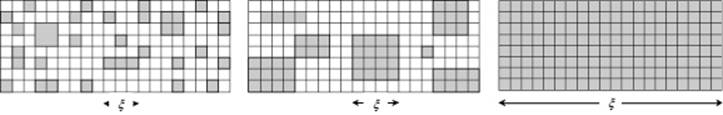
The next step in the elucidation-of-transitions process was provided by Kadanoff [8]. Essentially, the idea of scaling is applied to a lattice. One can think of the lattice gas model for which a Hamilton function describes the equilibrium distribution of occupied and nonoccupied lattice sites (see Appendix C). The correlation between the sites is given by the (total) correlation function h(r) ≡ ⟨ρ(r)ρ(0)⟩ − ⟨ρ²⟩, and we use the coherence length ξ as a measure of the range of the correlation function (Figure 16.9).

Figure 16.9 The coherence length ξ for the lattice gas model for (from left to right) T << T_cri, T < T_cri, and T = T_cri.

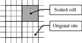
Consider therefore a D-dimensional lattice with N sites and lattice constant a and partition this lattice in cells (or blocks) of size La with L >> 1 (Figure 16.10). Hence, there are n = N/L^D cells, each containing L^D sites. Further consider that we are close to T_cri so that the correlation length ξ >> La. Next, we associate with each cell a parameter that states whether the cell as a whole is considered to be occupied, or not. For this process we use a definite rule. For example, in the case of averaging over three lattice sites in a triangular lattice, we obtain a cell for which we apply the majority rule, that is, a value of 1 is taken if at least two of three original sites have also the value 1. Hence, 000 → 0 (occurrence 1), 001 → 0 (occurrence 3), 011 → 1 (occurrence 3), and 111 → 1 (occurrence 1). Finally, we assume that for the cells the same Hamiltonian applies as for the sites. If that is the case then one might expect that the thermodynamics of the site model would be the same as that for the cell model. Denoting the relative temperature difference (with respect to T_cri) as before by t and the pressure by P, we have for a cell (site) t_cell (t_site) and P_cell(P_site). The Gibbs energy g per site or per cell of the site and cell model, respectively, then relate as

(16.74)

Figure 16.10 Lattice scaling illustrated for a 2D square lattice.

Now, we need relations between t_cell and t_site on the one hand, and P_cell and P_site on the other hand. We expect that the pressure of the cell model is proportional to the pressure of the site model, but the proportionality constant Bwill be dependent on L. The same assumption can be made for t. So we have

(16.75)

Although it is possible to continue without further assumptions [9], we assume that

(16.76)

with x and y arbitrary numbers (see Justification 16.1). This leads right away to

(16.77)

This expression, stating that g is a generalized homogeneous function of t and P, leads essentially to scaling with exponents p = x/D and q = y/D.

Justification 16.1: Power laws as scale-free functions

Since any dimensionless number can be raised to a certain power, one might ask why a power relation (x/x₀)^b is more scale-free than, say, an exponential relation exp(x/x₀), since for both a scale length x₀ is involved. Suppose that we have a power relation reading y/y₀ = a(x/x₀)^b, and that we have data available for the range x = x₀/2 to x = 2x₀. This implies that the ratio between maximum and minimum measured values is 4^b. If we scale x₀ to cx₀ and use the same range of data, we still have a factor of 4^b between maximum and minimum measured values. This implies that a superposition of these data ranges can be realized by a simple linear change of scale, and appears the same no matter on what scale it is probed. No other function is capable of doing this.