Liquid-State Physical Chemistry: Fundamentals, Modeling, and Applications (2013)

16.5. Renormalization

The plot thickens, as they say, and the next step is considerably more complex than the previous ones. That is why only a sketch of an answer to the remaining questions will be given. Full details can be found in the literature listed in the section labeled “Further Reading”.

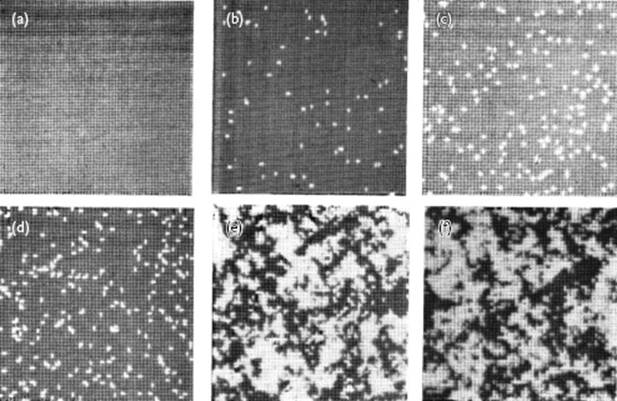
To continue, we need fluctuations for which in Figure 16.11 snapshots from an early Monte Carlo (MC) simulation of the 2D lattice gas model using 64 × 64 cells are shown. From these pictures and other evidence it became clear that, near T_cri, fluctuations occur on every length scale, and that the structure of the pictures is rather independent of the density, suggesting self-similar behavior. The coherence length ξ, which measures the range of the correlation function g(r), scales as ξ/ξ₀ ∼ |t|^−ν above as well as below T_cri. In order to have self-consistency, fluctuations in g(r) should be much smaller than ⟨ρ²⟩. We have ⟨ρ²⟩ ∼ t^2β and g(r) ∼ exp(−r/ξ)/r^D−2+η. Hence, for r ≅ ξ, we obtain t^2β > (t^−ν)^{−(D−2+η)} or, using Stanley's lemma, 2β < ν (D − 2 + η). Using scaling theory, this inequality also appears to be an equality. Using the mean field values β = ½, ν = ½ and η = 0, results in D ≥ 4. This result states that for fluctuations to be unimportant, the dimensionality should be at least four, which implies that in 3D, fluctuations do matter. One might think that adding fluctuations to the mean field result would remedy the situation, but since the fluctuations are more divergent than the mean values, this approach is not fruitful.

Figure 16.11 (a–c) The lattice gas model for T = 0, T = T_cri/4, T = T_cri/2; (d–f): The lattice gas model for T = 3T_cri/4, T ≅ T_cri, and T > T_cri. Images taken from Ref. [15].

The answers to the question of what are the numerical values of the critical exponents can be found in the approach, normally called the renormalization group (RG) theory [10]. In the simplest form of this theory we choose a transformation which transforms the original Hamiltonian of the site lattice with lattice constant a to a new Hamiltonian of the cell lattice with lattice constant La, without changing the expression for the partition function, that is, . Further, we use the usual lattice model approximation in which a site (cell) is occupied or not, representing repulsion, and only nearest-neighbor interactions with parameter J, representing attraction, are considered. In fact, this idea was used in the previous paragraph with respect to the Gibbs energy of the lattice, but here we employ the Hamiltonian. The basic idea is that this transformation can be described by r₁ = f(r) so that the parameters r₁ of the Hamiltonian of the cell lattice can be obtained from the parameters r of the Hamiltonian of the site lattice. This process can be iterated, that is, r₂ = f(r₁) = f[f(r)] and so on, for increasingly larger blocks until La reaches ξ. We can describe this process also by r_i+1 = f(r_i). It may happen that for i → ∞ we obtain r* = f(r*), where r* is called a fixed point. As an example we use the function

(16.78)

The fixed points are then the solutions of r* = cr*(1 − r*), which are r* = 0 and r* = 1 − 1/c. Stability can be probed by adding a small perturbation ε_i to r* so that x_i = r* + ε_i. From substitution in Eq. (16.78) and expanding f(r_i) in a Taylor series while keeping only the linear term, we obtain

(16.79)

If , then during each iteration the distance to r* will decrease and the fixed point will be called stable. If, on the other hand, , the distance will increase and the fixed point is called unstable. For our example, Eq. (16.78), df/dr = c(1 − 2r) and since c > 1, r* = 0 is an unstable fixed point and r* = 1 − 1/c is a stable fixed point.

From the above procedure we can determine not only the fixed points but also the way in which they are approached. Using r₁ = f(r), one obtains

(16.80)

Now, during the transformation the Gibbs energy per particle g(r) must be unaltered, that is, g(a₁) = L^Dg(a) or, equivalently, for the partition function . This scaling can only be done if the cell size is less than the coherence length ξ. Since for T → T_cri, ξ → ∞, at T_cri the scaling can be done for any cell size. Hence, we identify the critical point of the phase transition T_cri with the fixed point T*. Taking r = J/kT, with J the interaction energy and k Boltzmann's constant, we can rewrite Eq. (16.80), for r not too far removed from r*, as

(16.81)

On comparison with the general expression t₁ ≡ (T − T_cri)/T_cri = Lt, we obtain

(16.82)

If there are more parameters, say r = r(t) as before and s = s(P) (actually s = P/kT for the pressure ensemble), we have f = f(r,s) and we have two equations, namely

(16.83)

and using the same procedure we obtain

(16.84)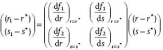

Because r₁ and s₁ are coupled, we transform to normal coordinates to obtain the scaling behavior, and for this we must find the eigenvalues of the derivative matrix. For convenience, we label the derivative matrix as T and denote the set (r − r*) and (s − s*) by the column δk, so that Eq. (16.84) reads δk₁ = Tδk. However, as T is non-symmetric⁹⁾, generally its left and right eigenvectors will be different. Using φ as the column for the left eigenvectors, we write , where the superscript α labels the eigenvalues λ. In spite of T being a non-symmetric matrix, the eigenvectors do not mix with one another under a RG transformation. This is readily shown by introducing the normal coordinates u^(α) = (φ^(α))^Tδk, from which one obtains

(16.85)

If we assume that all eigenvalues are real, the local geometry of the Hamiltonian surface around a fixed point is thus described by the normal coordinates u^(α), which are moreover scale-invariant. This implies that the Hamiltonian and therefore the Gibbs energy per particle g(k) can be written in terms of the normal coordinates u^(α). We write g(u⁽¹⁾,u⁽²⁾, …) = b^−Dg(λ⁽¹⁾u⁽¹⁾, λ⁽²⁾u⁽²⁾, …), and we identify the coordinates u^(α) as the scaling parameters of the problem. Since in general at T_cri all u^(α) are zero, we can determine for a given coordinate, say number 1, its behavior close to T_cri, by setting u⁽²⁾, u⁽³⁾, … equal to zero so that we have g(u⁽¹⁾,0, …) = L^−Dg(λ⁽¹⁾u⁽¹⁾, 0, …). If only r = r(t) and s = s(P) are the variables of interest, we have g(r,s) = L^−Dg(λ⁽¹⁾r, λ⁽²⁾s) and comparing this expression with the Widom scaling function g(λ^pt,λ^qP) = λg(t,P) the result becomes

(16.86)

In Section 16.4 we have shown that all exponents follow from p and q. Hence, all critical exponents are determined by the scaling behavior of the eigenvalues of the linearized transformation matrix T near the critical point.

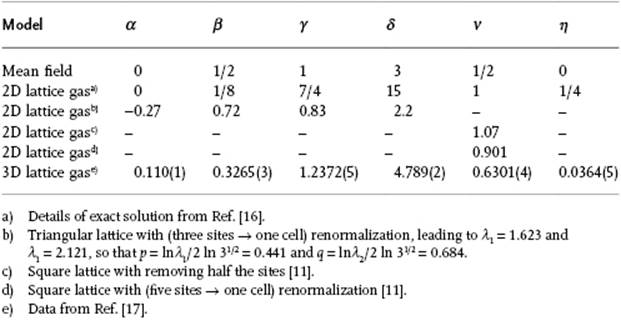
Applying this process, the critical exponents of the lattice model have been obtained to high accuracy (Table 16.4). As an illustration of the accuracy of some approximate results, the values for the 2D lattice gas using different lattices and blocks are also given. Note the good agreement of the 3D values as calculated using renormalization theory with the experimental values (Table 16.3). To conclude this part, we note that the above-outlined procedure is the simplest possible way of renormalizing real space. Moreover, we note that the inverse of these trans­formations does not exist, so that the designation “renormalization group” actually should read “renormalization semi-group.” However, the nomenclature is conventional.

Table 16.4 Critical exponents according to various models.

This approach is apparently abstract and we refrain from detailing one or another model. It may be useful, however, to illustrate the methods by a much simpler example, namely that of percolation [12]. If we mix electrically conducting and insulating particles at random, using an increasing fraction of conducting particles, the mixture will at first be insulating; however, at a certain fraction a transition to a conductive mixture will occur. This change occurs over a small volume fraction change of conductive particles, and thereafter the conductivity still increases, albeit slowly. This phenomenon is called percolation, and the transition is termed the percolation threshold. The phenomenon can be considered as a geometric phase transition where, at the percolation threshold infinite, connected clusters of conductive particles will appear. For 2D (i.e., for disks) the transition occurs at 50 vol.%, whereas for 3D (i.e., for spheres), it occurs at about 16 vol.%. The development of these clusters in the percolation model is similar to that of clusters of molecules in phase transformations. Each realization of a packing at a certain volume fraction can be considered as a snapshot of a configuration of two types of molecule. Of course, the analog is static in time, but the basic idea is the same.

The physical problem is now to derive when and how electrical conduction across a macroscopic region occurs, in terms of the microdetails of the packing of the particles. As a concrete example, we use a 2D structure with a renormalization by three particles (disks). For the original packing the microdescription is in terms of sites that are either occupied or unoccupied with a conductive particle. We denote the probability that any site is occupied by p, independent of whether any other site is occupied, or not. The occupancy distribution of sites provides the exact microdescription of the system for which we only know the single site probability p.

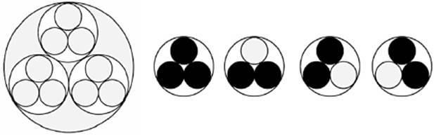
In the spirit of the renormalization theory, we increase the length scale by b, that is, we increase the area by b² = 3. At the higher level of description, in this case a cell of three sites, and using the majority rule, a cell will be occupied if, and only if, two or more of the sites are occupied (Figure 16.12). Let us call p₁ the probability that a cell of three sites is occupied. The probability p₁ is then the sum of probabilities of four mutually exclusive states. Using p for occupied sites and (1 − p) for unoccupied sites, we have once p³ and three times p²(1 − p).

Figure 16.12 Percolation and renormalization by taking three spheres together, to which the majority rule is applied. The left schematic shows the original packing; the smaller schematics (at right) show the four possible “renormalized” sites.

The percolation threshold (critical point) occurs if the original probability p equals the renormalized probability p₁. We thus have

(16.87)

The solution of this equation does not require iteration but yields directly as solutions p* = 0 and p* = 1 which represent the stable fixed points, and the solution p* = 0.5 representing the unstable fixed point. The unstable fixed point solution thus appears to be the exact solution for this 2D percolation problem, which however, is fortuitous.

Let us now calculate the critical exponent ν which describes the onset of the percolation phenomenon. We take the coherence length ξ for the original packing to be given by ξ = C|p − p_cri|^−ν, while for the renormalized packing we have ξ₁ = C|p₁ − p_cri|^−ν with ξ₁ = ξ/b. Combining results in

(16.88)

(16.89)

Expanding p₁ as p₁ = p* + λ*(p − p*) + … with and substitution in the original equation p₁ = p³ + 3p²(1 − p) yields

(16.90)

so that λ* = 3/2. Because b² = 3, we obtain

(16.91)

The exact value is ν = 4/3. Approaching the threshold, the coherence length ξ of the clusters increases until ξ diverges at the threshold itself. This implies that conductive clusters span the complete system and therefore become macroscopically conductive.

Problem 16.10

Show that for T′ − T* << T*, Eq. (16.80) is equivalent with Eq. (16.81).

Problem 16.11*

Show that the scaling relation for conduction percolation on a BCC lattice reads p₁ = p⁹ + 9p⁸(1 − p) + 36p⁷(1 − p)² + 84p⁶(1 − p)³ + 126p⁵(1 − p)⁴. If you feel up to it, obtain the percolation threshold p* and the critical exponent ν.