March's Advanced Organic Chemistry: Reactions, Mechanisms, and Structure, 7th Edition (2013)

This book contains 19 chapters. Chapters 1–9 may be thought of as an introduction to Part II. The first-five chapters deal with the structure of organic compounds. These chapters discuss the kinds of bonding important in organic chemistry, the fundamental principles of conformation and stereochemistry of organic molecules, and reactive intermediates in organic chemistry. Chapters 6–9 are concerned with general principles of mechanism in organic chemistry, including acids and bases, photochemistry, sonochemistry and microwave irradiation, and finally the relationship between structure and reactivity.

Chapters 10–19, which make up Part II, are directly concerned with the nature and the scope of organic reactions and their mechanisms.

Chapter 1. Localized Chemical Bonding

Localized chemical bonding may be defined as bonding in which the electrons are shared by two and only two nuclei. Such bonding is the essential feature associated with the structure of organic molecules.¹ Chapter 2 will discuss delocalized bonding, in which electrons are shared by more than two nuclei.

1.A. Covalent Bonding²

Wave mechanics is based on the fundamental principle that electrons behave as waves (e.g., they can be diffracted). Consequently, a wave equation can be written for electrons, in the same sense that light waves, sound waves, and so on, can be described by wave equations. The equation that serves as a mathematical model for electrons is known as the Schrödinger equation, which for a one-electron system is

where m is the mass of the electron, E is its total energy, V is its potential energy, and h is Planck's constant. In physical terms, the function (Ψ) expresses the square root of the probability of finding the electron at any position defined by the coordinates x, y, and z, where the origin is at the nucleus. For systems containing more than one electron, the equation is similar, but more complicated.

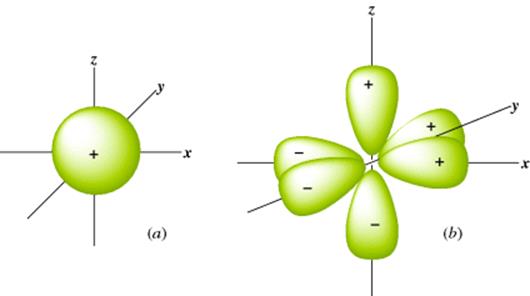
The Schrödinger equation is a differential equation, so solutions to it are themselves equations, but the solutions are not differential equations. They are just simple equations for which graphs can be drawn. Such graphs are essentially three-dimensional (3D) pictures that show the electron density, and these pictures are called orbitals or electron clouds. Most students are familiar with the shapes of the s and p atomic orbitals (Fig. 1.1). Note that each porbital has a node: A region in space where the probability of finding the electron is extremely small.³ Also note that in Fig. 1.1 some lobes of the orbitals are labeled + and others −. These signs do not refer to positive or negative charges, since both lobes of an electron cloud must be negatively charged. They are the signs of the wave function Ψ. When a node separates two parts of an orbital, a point of zero electron density, Ψ always has opposite signs on the two sides of the node. According to the Pauli exclusion principle, no more than two electrons can be present in any orbital, and they must have opposite spins.

Fig. 1.1 (a) The 1s orbital. (b) The three 2p orbitals.

Unfortunately, the Schrödinger equation can be solved exactly only for one-electron systems (e.g., the hydrogen atom). If it could be solved exactly for molecules containing two or more electrons,⁴ a precise picture of the shape of the orbitals available to each electron (especially for the important ground state) would become available, as well as the energy for each orbital. Since exact solutions are not available, drastic approximations must be made. There are two chief general methods of approximation: the molecular orbital (MO) method and the valence bond method.

In the MO method, bonding is considered to arise from the overlap of atomic orbitals. When any number of atomic orbitals overlap, they combine to form an equal number of new orbitals, called molecular orbitals. Molecular orbitals differ from atomic orbitals in that an electron cloud effectively surrounds the nuclei of two or more atoms, rather than just one atom. In other words, the electrons are shared by two atoms rather than being localized on one atom. In localized bonding for a single covalent bond, the number of atomic orbitals that overlap is two (each containing one electron), so that two molecular orbitals are generated. One of these, called a bonding orbital, has a lower energy than the original atomic orbitals (otherwise a bond would not form), and the other, called an antibonding orbital, has a higher energy. Orbitals of lower energy fill first. Since the two original atomic orbitals each held one electron, both of these electrons will reside in the new molecular bonding orbital, which is lower in energy. Remember that any orbital can hold two electrons. The higher energy antibonding orbital remains empty in the ground state.

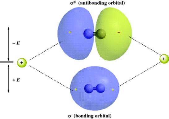
The strength of a bond is determined by the amount of electron density that resides between the two nuclei. The greater the overlap of the orbitals, the stronger the bond, but total overlap is prevented by repulsion between the nuclei. Figure 1.2 shows the bonding and antibonding orbitals that arise by the overlap of two 1s electrons. Note that since the antibonding orbital has a node between the nuclei, there is practically no electron density in that area, so that this orbital cannot be expected to bond very well. When the centers of electron density are on the axis common to the two nuclei, the molecular orbitals formed by the overlap of two atomic orbitals are called σ (sigma) orbitals, and the bonds are called σ bonds. The corresponding antibonding orbitals are designated σ∗. Sigma orbitals may be formed by the overlap of any of the atomic orbital (s, p, d, or f) whether the same or different, not only by the overlap of two s orbitals. However, the two lobes that overlap must have the same sign: A positive s orbital can form a bond only by overlapping with another positive s orbital or with a positive lobe of a p, d, or f orbital. Any σmolecular orbital may be represented as approximately ellipsoidal in shape.

Fig. 1.2 Overlap of two 1s orbitals gives rise to a σ and a σ∗ orbital.

Orbitals are frequently designated by their symmetry properties. The σ orbital of hydrogen is often written ψ_g. The g stands for gerade. A gerade orbital is one in which the sign on the orbital does not change when it is inverted through its center of symmetry. The σ^∗ orbital is ungerade (designated ψ_u). An ungerade orbital changes sign when inverted through its center of symmetry.

In MO calculations, the linear combination of atomic orbitals (known as LCAO) generates a wave function from a linear combination of overlapped atomic orbitals. Addition of the atomic orbitals gives the bonding MO:

(1-1)

The functions ψ_A and ψ_B are the functions for the atomic orbitals of atoms A and B, respectively, and c_A and c_B represent weighting factors. Subtraction is also a linear combination:

(1-2)

This gives rise to the antibonding molecular orbital.

In the valence bond method, a wave equation is written for each of various possible electronic structures that a molecule may have (each of these is called a canonical form), and the total ψ is obtained by summation of as many of these as seem plausible, each with its weighting factor:

(1-3)

This resembles Eq. (1-1), but here each ψ represents a wave equation for an imaginary canonical form and each c is the amount contributed to the total picture by that form. For example, a wave function can be written for each of the following canonical forms of the hydrogen molecule⁵:

Values for c in each method are obtained by solving the equation for various values of each c, and choosing the solution of lowest energy. In practice, both methods give similar solutions for molecules that contain only localized electrons, and these are in agreement with the Lewis structures long familiar to the organic chemist. Delocalized systems are considered in Chapter 2. Note that orbital functions can indeed be reconstructed from measured data using several different approaches. Often, however, the results are still less accurate than those achieved with purely theoretical methods.⁶