Physical Chemistry Essentials - Hofmann A. 2018

Interactions of Matter with Radiation
13.2 Magnetic Resonance Spectroscopy

13.2.1 General Principles

As we have seen in Sect. 10.2.2, an electron rotating around its own axis (spin) constitutes a charged particle in motion, leading to a magnetic spin momentum which is characterised by the magnetic spin quantum number m _s . As a consequence, the electron spin is oriented with respect to an external magnetic field (see Fig. 10.8).

If we consider atomic nuclei, it is obvious that these are charged particles, too, and, upon rotation around their own axis there is a resulting nuclear spin momentum the value of which is given as

(13.16)

introducing the nuclear spin quantum number I. Whereas the electron spin quantum number s assumes only value (½), the value of the nuclear spin quantum number I is not as tightly restricted and, in general, cannot be predicted; values between 0 and 8 have been observed so far. Whereas protons and neutrons (the components constituting the atomic nucleus; also called nucleons) each have net spins of ½, there are also spin interactions among the elementary particles ( quarks) that, in turn, compose the nucleons. As a result of this complexity, there is no simple formula to predict I based on the number of protons and neutrons within an atom. However, there are three main rules:

✵ If the number of protons (Z) as well as the number of neutrons (N) is even, the nuclear spin quantum number I is zero. For example, ¹²C and ¹⁶O possess no nuclear spin.

✵ If Z is even and N odd, or vice versa, then I is half-integral. For example, the nuclear spin quantum number of ¹H, ¹³C, ¹⁵N, ¹⁹F and ³¹P is I = ½.

✵ If both Z and N are odd, then the nuclear spin quantum number takes an integral value. For example, ²H and ¹⁴N have I = 1.

If either an electron or a nucleus with their respective spins are exposed to an external magnetic field , then the spins need to orient themselves such that the space component of the electron spin () or nuclear spin () can only take the following values (Table 13.2):

Table 13.2

Comparison of electron and nuclear spin directions in an external magnetic field

An external magnetic field will exert a torque on a magnetic dipole and, therefore, the potential energy of both electrons and nuclei includes a magnetic component which is given as the product between the magnetic momentum of either electron or nucleus and the magnetic field itself:

(13.17)

The magnetic momentum is derived from the spin quantum numbers m _s (electron) and m _I (nucleus):

We appreciate that in this derivation, the use of a gyromagnetic ratio (also called g-factor) is introduced. The g-factor for an orbital is g _l = 1, but for the electron spin a factor of g_e ≈ 2 has been found. For nuclei, the g-factor depends on the individual element; measurements for the protein and neutron yielded that

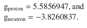
Surprisingly, the g-factor for the neutron is far from zero, despite the neutron does not carry a charge! This indicates that inside the neutron there is an internal structure involving the movement of charged particles (the elementary particles called quarks).

Table 13.3 also introduced the magnetons which are units of the magnetic momentum. For the electron, this yields the Bohr magneton μ_B, and for nuclei units of nuclear magnetons μ_N are commonly used. The quantisation of electron and nuclear magnetic momentum thus yields equally spaced energy levels.

Table 13.3

Comparison of the potential magnetic energy of electrons and nuclei

As an illustration, we will calculate the the potential magnetic energy difference for the two magnetic spin states of the electron (m _s = ±¹/₂) as well as the the two nuclear spin states of the proton (m _I = ±¹/₂) in the presence of an external magnetic field . For the electron, this yields:

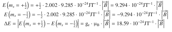
(13.18)

The same evaluation yields for the proton:

(13.19)

We see, firstly, that whereas for the electron the state m _s = −¹/₂ is energetically favoured, for the proton it is the state with m _I = +¹/₂. Second, assuming the same strength of the externally applied magnetic field, the difference between both energy levels is much larger for electrons than for protons.

In the introduction to this chapter, we discussed that in order to elicit a transition from a just the difference in energy between the two states the spin momentum component, i.e. satisfies the resonance condition. Assuming an external magnetic field of 2.0 T, the energy required for proton spin resonance would thus be:

which is in the region of radio waves.

We can thus conclude that in order to satisfy the nuclear magnetic resonance condition, electromagnetic radiation in the range of radio waves will be required. Since the energy difference of the magnetic electron spin levels is three orders of magnitude higher (at the same magnetic field strength), radiation in the microwave range will satisfy the resonance condition for electron spin resonance. In principle, the resonance condition can in both cases be achieved by either applying a constant magnetic field and variation of the frequency ν of the incident electromagnetic radiation, or a constant frequency and variation of the magnetic field .

Using the Boltzmann expression introduced in Sect. 13.1.2, it is possible to calculate the ratio of populations of the lower and the higher energy states of electron and nuclear spins in the presence of an external magnetic field (Table 13.4). Owing to the small energy differences between higher and lower states, the differences in population of both states are extremely small. Provision of the resonance energy ΔE by incident electromagnetic radiation leads to a change of the population ratio as the energetically higher spin states are increasingly populated after absorption of ΔE.

Table 13.4

Comparison of the ratio of populations of lower and higher states for electron and nuclear spin using the energy differences from Eqs. 13.18 and 13.19 at a temperature of T = 300 K

For the comparison in Table 13.4, we have used the field strength of the external magnetic field supplied by the instrumentation used for electron spin resonance or nuclear magnetic resonance spectrometry. A closer look at the observed phenomena shows that the field strength experienced by a particular electron or nucleus in a molecule does not exactly equal the the field strength of the external magnetic field but is slightly different. Since the electron density varies with the type of chemical bond, the observed resonance is shifted with respect to the position expected based on the external magnetic field strength. This shift is also called chemical shift and constitutes an important parameter when deducing the chemical structure from magnetic resonance spectra.

After the absorption of the resonance energy caused an increase in the population of the higher spin states, the reverse process occurs whereby spins return to the lower energy state—this is known as relaxation. The population ratio N _high:N _low returns to values determined by the presence of the external magnetic field (see Table 13.4). The energy released during those transitions is dissipated into the environment (’lattice’) as heat. This process happens with a kinetics of first order and has a rate known as spin-lattice relaxation time or longitudinal relaxation time T ₁. The rate constant is, accordingly, T ₁ ⁻¹.

A related phenomenon is observed for the phases of the spins. After turning on the magnetic field, the movement of all spins are in phase, but the exchange of energy between spins, inhomogeneous/disturbed local magnetic fields as well as the spin-lattice relaxation all lead to a decrease in the phase correlation of spin movements. This process also happens with a kinetics of first order and is described by the transversal (sometimes also called spin-spin) relaxation time T ₂.

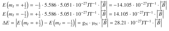
Both T ₁ and T ₂ are characteristic parameters for the life time of the excited state and thus affect the peak width observed in magnetic resonance spectra. A brief comparison is summarised in Table 13.5 (Fig. 13.7).

Table 13.5

Comparison of T ₁ and T ₂ relaxation

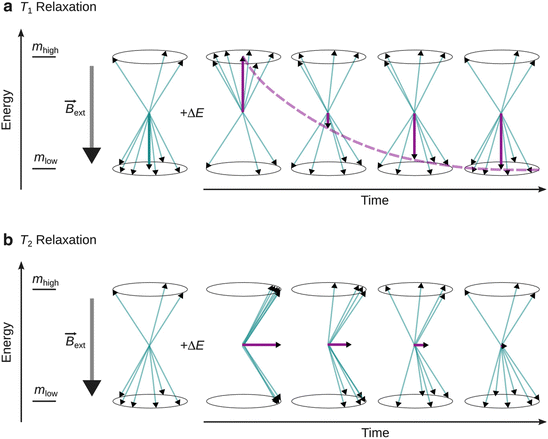
Fig. 13.7

Illustration of T ₁ and T ₂ relaxation. ’+ΔE’ indicates provision of the resonance energy. (a) T ₁ or longitudinal relaxation leads to a decrease of the magnetisation anti-parallel to the external magnetic field. (b) T ₂ or transversal relaxation results in decrease of magnetisation orthogonal to the external magnetic field

13.2.2 Nuclear Magnetic Resonance (NMR) Spectroscopy

NMR spectroscopy requires a strong homogeneous magnetic field which is provided in contemporary spectrometers by superconducting magnets (currently up to 23.5 T equivalent to a resonance frequency of 1 GHz). Historically, the early spectrometers operated in the so-called continuous wave method and used electromagnets. A sweep generator was used for sweeping either the magnetic or radio frequency field through the resonance frequencies of the sample. Contemporary spectrometers are operated as Fourier Transform NMR spectrometers where all required radio frequencies are transmitted at once in a radiation pulse and cause nuclei in the magnetic field to flip into the higher-energy alignment (so-called pulse-acquire method). In the following time T, the nuclei return to their original states and emit a radio frequency signal called the free induction decay (FID). The FID contains all the resonance signals of the sample, but they are coded in the time domain. With the computational process of Fourier transformation, these data can be converted into a conventional spectrum where the resonance intensities are ordered per frequency. For illustration, we will focus on proton (¹H) NMR to discuss some general principles of this spectroscopic method.

When considering the energy difference between the higher and lower proton spin states as derived in Eq. 13.19, one needs to be aware that the value of in that equation is not the strength of the external magnetic field , but the local magnetic field experienced at the position of the nucleus. The local field strength is less than , since the orbiting electrons generate a magnetic field counteracting the external magnetic field. The orbital motion of electrons around a nucleus creates constitutes current loops, which produce magnetic fields of their own. In the presence of an external magnetic field, these current loops will align in such a way as to oppose the applied field. Macroscopically, this effect may be illustrated by a tiny magnet that is brought into an external magnetic field; the small magnet will align itself such that its field is opposed to the external magnetic field (Fig. 13.8). The lesser magnetic field exhibited by a particular nucleus therefore leads to a lesser resonance energy which is called the chemical shift. Since the electron density in a molecule varies with location, depending on the chemical bonds, different chemical shifts are observed for different bonding situations.

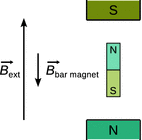
Fig. 13.8

The field of small magnets experiencing an external magnetic field opposes the direction of the external field

Since the registered chemical shifts are extremely small compared to the external magnetic field, NMR spectra are not plotted against the effective magnetic field strength but rather compared to an internal standard; for ¹H-NMR this is typically tetramethylsilane (TMS) which produces a single peak in a proton NMR experiment. The chemical shift δ is defined as

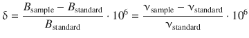
(13.20)

and therefore yields δ = 0 ppm for the standard. Figure 13.9 shows the ¹H-NMR spectrum of 1-chloropropane which features three clusters of peaks. The step-type curves show the integration of the individual peak clusters (i.e. peak areas). The integration values form the ratio 2:2:3 which indicates that the peak clusters originate from the ClCH₂−, the −CH₂− and the CH₃-group with 2, 2 and 3 protons, respectively. The fine structure in each peak cluster demonstrates the substantial impact of the local environment and is thus an extremely important part of structure determination.

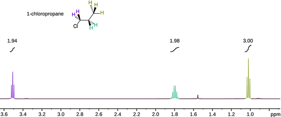
Fig. 13.9

¹H-NMR spectrum of 1-chloropropane acquired in CDCl₃ at room temperature on a Bruker 500 MHz Avance III NMR spectrometer at room temperature. Each peak cluster has been integrated and the numerical values are shown above the integration curves. (Spectrum courtesy of Dr Siji Rajan.)

As evident from Fig. 13.9, the ¹H-NMR spectrum of 1-chloropropane shows a triplet peak for the methyl group (δ = 1.02 ppm). This is due to the coupling of the spin of methyl protons with the spins of neighbouring methylene protons ( spin-spin coupling). With two possible spins for each methylene proton, the spin of a methyl proton can couple with four different combinations of methylene proton spin orientations; however, two of those combinations are indistinguishable and thus collapse into one peak (Fig. 13.9).

The methylene proton spins experience the the spin configurations of the methyl group of which there are eight different. However, there are three indistinguishable configurations each that possess a total spin of +¹/₂ and −¹/₂, respectively. The splitting pattern of the methylene protons thus yields a quartet. Additionally, the methylene proton spins can also couple with the spins of the chloromethyl protons (three distinct possible orientations) which leads to a triplet splitting of each of the quartet peaks. This results in a complex multiplet that is difficult to resolve and appears as a sextet (δ = 1.80 ppm). The two protons of the chloromethyl group split into a triplet pattern (δ = 3.51 ppm) as their spins experience the spin combinations of the two methylene protons.

The separation between the lines of a multiplet yields the spin-spin coupling constant J. The magnitude of the coupling constant is determined by the extent of the magnetic interaction between two nucleic spins. There are three important observations regarding proton spin-spin coupling:

✵ Nuclei that have the same chemical shift (i.e. they constitute equivalent nuclei) do not interact with each other in this manner.

✵ Coupling occurs primarily between protons that are separated by three bonds; the number of bonds between two coupling nuclei is indicated by a subscript on the coupling constant (e.g. ²J, ³J, …).

✵ Coupling is most noticeable with protons bonded to carbon (Fig. 13.10).

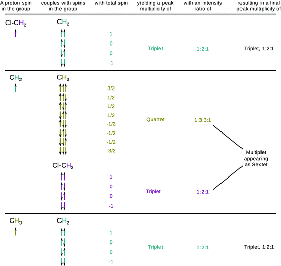
Fig. 13.10

Proton spin-spin couplings in 1-chloropropane

13.2.3 Electron Spin Resonance (ESR) Spectroscopy

ESR (also called electron paramagnetic resonance or EPR) spectroscopy shares the general concepts with NMR spectroscopy and both methods therefore have many features in common. In ESR spectroscopy, a sample is exposed to a homogeneous external magnetic field which leads to a slight over-population of the lower spin state (see Table 13.4). The energy difference ΔE between the lower and higher spin state is overcome by provision of electromagnetic radiation that satisfiers the resonance condition. In Sect. 13.2.1 we have seen, that the energy difference between the two spin states of the electron is about three orders of magnitude larger than in case of the nuclear spin states. Using Eq. 13.18 and assuming an external magnetic field of 0.5 T, the energy required for electron spin resonance is:

which is in the region of microwaves.

Importantly, only molecules that possess an unpaired electron are amenable to ESR spectroscopy, since paired electrons cannot undergo a change of spin as this would violate the Pauli exclusion principle (see Sect. 10.3.2). Therefore, ESR spectroscopy is limited to the investigation of radical species of which there are naturally only few. However, the use of so-called spin-labels—chemical groups with a stabilised radical that can be covalently attached to molecules of interest—allows the investigation of many processes by means of the attached reporter group carrying an unpaired electron. ESR spectroscopy with spin labels is a frequently used method in the biosciences to study processes on and around proteins and membranes. Only two transitions are allowed for the unpaired electron, though, as is reflected by the selection rules:

(13.21)

The rule demanding conservation of the nuclear spin (Δm _I = 0) can be explained if one assumes that the motion of a nucleus is much slower than that of an electron. In other words, in the time it takes for the electron to change its spin (Δm _s = ±1), the nuclear spin has no time to reorient.

For practical reasons, ESR spectra don’t register the absorption peak but rather its first derivative (Fig. 13.11). For free electrons, the ESR spectrum contains just one peak. If we consider the hydrogen atom, which constitutes the simplest radical consisting of one proton and one electron, we find that the ESR spectrum shows two peaks with the same intensity; the distance between both peaks is measured at 50.7 milli-tesla (mT). For comparison, the signal of the free electron comes to lie in the centre between the two peaks of the hydrogen atom. Similar to the observations made in nuclear magnetic resonance, the spin signal of the hydrogen electron is split into a doublet.

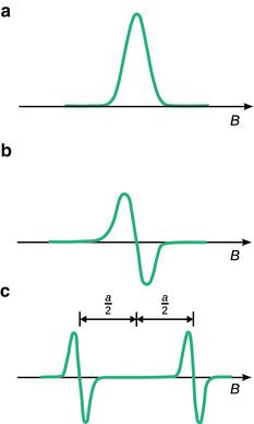
Fig. 13.11

(a) ESR absorption signal of an unpaired electron, and (b) its first derivative. (c) The hyperfine splitting of the ESR signal of the unpaired electron in the hydrogen atom shows a doublet with a coupling constant of a ^H = 50.7 mT

The splitting is the result of an interactions between the spin of the unpaired electron and the nuclear spin, known as the Fermi contact. This interaction only arises when the unpaired electron is inside the nucleus—a phenomenon that can only be explained using the probability density (introduced in Sect. 8.3.2):

(8.32)

The effect of the nuclear magnet on the spin of the unpaired electron can be summarised in form of an additional magnetic field (contact field), which depends on the magnetic moment of the nucleus (given by the quantum number m _I ), the g-factor of the nucleus (g_N), the nuclear magneton (μ_N), as well as the spin density of the unpaired electron in the nucleus (|Ψ|²):

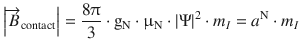
(13.22)

thereby defining the hyperfine coupling constant a ^N.

For the proton, the probability density of the electron in the 1s orbital can be calculated, thereby allowing the computation of a theoretical hyperfine coupling constant for the hydrogen atom. The calculated value of a ^H = 50.8 mT is in excellent agreement with the experimentally observed value of 50.7 mT.

If the unpaired electron of a radical interacts with two different (non-equivalent) nuclei, for example protons H1 and H2, a more complex splitting pattern arises due to independent nuclear spin orientations of both protons. Interaction of the electron with H1 leads to a doublet pattern with a coupling constant of a ^H1 as discussed above. Due to the presence of H2, one needs to consider that each of those situations can also show coupling with the nuclear spin orientations of H2, which possesses a different coupling constant a ^H2. The hyperfine splitting therefore results in ’doublet of doublet’ pattern where all peaks possess the same intensity (Fig. 13.12 left). Notably, if the electron was to interact with two equivalent protons (e.g. in the formyl radical H₂CO⁻), then the coupling constants a ^H1 and a ^H2 have the same value and the two centre peaks collapse into one peak. The resulting pattern of the hyperfine splitting thus appears as a triplet with intensity ratio 1:2:1 (Fig. 13.12 right). Generally, the number of hyperfine lines can be predicted as per

(13.23)

where N is the number of chemically equivalent nuclei and I is the nuclear spin.

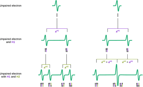
Fig. 13.12

Hyperfine splitting by coupling of an unpaired electron with two non-equivalent protons (left) and two equivalent protons (right)