5 Steps to a 5: AP Macroeconomics 2017 (2016)
STEP 4
Review the Knowledge You Need to Score High
CHAPTER 7
Macroeconomic Measures of Performance
Technically, this is the first chapter in the review of macroeconomics, but both AP Microeconomics and Macroeconomics courses begin with coverage of “Basic Economic Concepts,” a section that includes the following topics:
• Scarcity, choice, and opportunity costs
• Production possibilities curve
• Comparative advantage, specialization, and exchange
• Demand, supply, and market equilibrium
IN THIS CHAPTER
Summary: Should we raise or lower interest rates? Should we cut or increase taxes? The media is always buzzing about some macroeconomic policy intended to make our lives better. What does it mean to do better? How is “better” measured in something as large and complex as the macroeconomy? In general, macroeconomic policies share the goal of stabilizing and improving the economy, and they also share reliance upon statistical measures of economic performance. Though “statistics” might sound like a dirty word to you and your classmates, as AP Macroeconomics test takers, you need to understand how some important measures are, well, measured. Knowing how they are measured provides you with a much better way of responding to exam questions that ask you to use theoretical models to fix a macroeconomic problem. You cannot speak intelligently about growing the economy until you know how economic growth is measured. Likewise, if you want to perform better on the AP Macroeconomics exam, you might want to know exactly how those statistics (your grade) are compiled and study accordingly. This chapter introduces measurement of economic production and paves the way for models of the macroeconomy and policies intended to improve this economic performance.

Key Ideas
![]() The Circular Flow Model
The Circular Flow Model
![]() Gross Domestic Product
Gross Domestic Product
![]() Real versus Nominal
Real versus Nominal
![]() Inflation and the Consumer Price Index
Inflation and the Consumer Price Index
![]() Unemployment
Unemployment
7.1 The Circular Flow Model
Main Topic: Circular Flow Model of a Closed Economy
The Circular Flow Model
“What comes around goes around.” If you remember nothing else about the circular flow model, remember this old phrase. The circular flow of goods and services (or circular flow of economic activity ) is a model of an economy showing the interactions among households, firms, and government as they exchange goods and services and resources in markets. In other words, it is a game of “follow the dollars.”
Figure 7.1 illustrates a model of a closed economy , where the foreign markets are not assumed (yet) to exist. Domestic households offer their resources to firms in the resource market so that those firms can produce goods and services. The households are paid competitive prices for those resources. They use that income to consume the very goods that were produced through the employment of their productive resources. Revenues from the sale of goods and services are then used to provide income to those households. In this simplified model, every dollar of income in the household ends up as revenue for the firm.
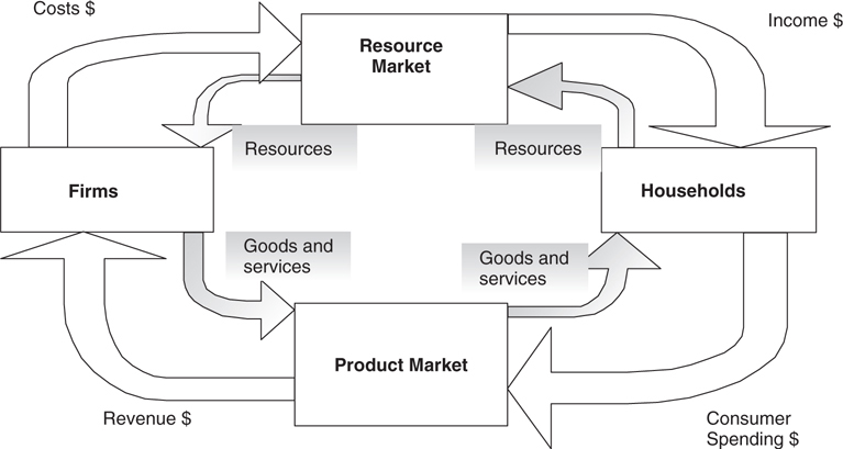
Figure 7.1
“What About the Government?”
Though not pictured in Figure 7.1 , the government plays an important role in the circular flow model. The government is an employer of inputs and a producer of goods and services. The government collects taxes both from households and firms and uses the funds to pay for the inputs that they employ.
“How Much Economic Activity Is Being Generated?”
We can add up all of the dollars earned as income by resource owners, or we can add up all of the spending done on goods and services, or we can add up the value of all of those goods and services.
“Where Does It Begin, Where Does It End?”
It doesn’t matter; it’s the counting of the dollars that is the important first step in measuring economic performance.
Macroeconomic Goals
Figure 7.1 implies that a steady flow of goods and dollars circulating throughout the economy is necessary or commerce ceases. The big issue is how we keep this flow strong, and how we know when it is weak. Measuring success is the focus of the sections that follow. Most modern societies maintain the fairly broad goal of keeping spending and production in the macroeconomy strong without drastically increasing prices.
7.2 Accounting for Output and Income
Main Topics: Valuing Production, Gross Domestic Product (GDP), National Income Concepts, Real and Nominal GDP, The GDP Deflator, Business Cycles
Valuing Production
The key here is to measure the value of the goods that are produced, not just the amount of goods that are produced. Remember the circular flow? If we need to follow the dollars to measure economic activity, we need to know prices of these goods.
Value of Production, Not Just Production
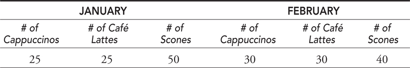
When you track the monthly production of a small coffee shop, you could sum up all of the cappuccinos, café lattes, and scones that were purchased. Table 7.1 represents the output in two recent months. At first glance, the two months produced the same amount (100) of goods, but clearly the mix of goods at the coffee shop is different.
Table 7.1 Production
Valuing Production
To paint a more accurate picture of production, we need to incorporate the value of these items as shown in Table 7.2 .
Table 7.2
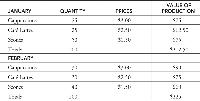
While the total production at the coffee shop remained the same from month to month, the value of that production has increased in February. There are now more dollars circulating.

• Don’t just add up the quantities; multiply by prices and add up the values.
Gross Domestic Product (GDP)
Aggregation, Not Aggravation
To move from valuing production of one firm to the entire town, to the state, or to the U.S. economy, we need to aggregate . Simply stated, we need to value all production of all firms and then add them up to get the value of production for the entire domestic economy. It is this aggregated measure of the total value of domestic production that allows us to calculate our first important macroeconomic statistic, GDP . GDP is the market value of the final goods and services produced within a nation in a year. If the good or service is produced within the borders of the United States, it counts toward U.S. GDP. It does not matter if the firm is headquartered in Indonesia; so long as it is producing in Indiana, it appears in the U.S. GDP.
What’s In, What’s Out
Final goods are those that are ready for consumption. A bottle of ketchup at the Piggly Wiggly is counted. Intermediate goods are those that require further processing before they are counted as a final good. When the tomatoes used to make ketchup are purchased from a grower, they are not counted toward the GDP. At least not until those tomatoes, and their value, find themselves in a bottle of ketchup and sold at the supermarket. A raw material like a tomato might be bought and sold several times before it appears as a final product. If we were to count the dollars at every stage of this process, we would be double counting, and this is to be avoided. Suppose the tomatoes go through three stages: harvest, processing, and retail sale as a bottle of ketchup. Along the way a pound of tomatoes is sold, bought, and altered. The pound of tomatoes was sold from the grower to the processor for 50 cents. The bottle of ketchup was sold to a grocery store for $1.50, and eventually the ketchup was sold to a consumer for $3. If we added all of these transactions, we come up with $5, which overstates the value of the good in its final use. GDP only adds the final transaction as the value of the final good produced and consumed.
Second-hand sales are not counted. This falls under the “do not double count” rule. If you buy a new Xbox at Best Buy in 2012, it would count in the GDP for 2012. If you resell it on eBay in 2015, it is not counted again. Final goods and services are only counted once, in the year in which they were produced.
Nonmarket transactions are not counted toward GDP. For example, if I have a clogged drain in my kitchen, I have two choices: fix it myself or call the plumber and pay to have it fixed. Doing it myself does not contribute to GDP, but paying a plumber to do it does. The same job is done, but only the latter ends up in the books. In a similar way, regular housework done at home by an unpaid member of the household is not counted, though it is very much a productive effort. This reality is sometimes cited as a criticism of GDP accounting: some valuable services are counted and others are not.
Underground economy transactions are not counted. For obvious reasons, the illegal sale of goods or services or paying someone cash “under the table” for work are not counted. Informal bartering between individuals is also not counted. You might help a friend study for economics, while she helps you study for biology, but this kind of bartering would not appear on any official ledger of production, even though it might be quite productive.
As a practical matter, official tabulation of GDP is never 100 percent accurate because the value of final goods and services is based upon a survey of representative firms, not a complete census of all firms throughout the nation. Despite this methodology, economists work very hard to get a fairly accurate picture of the value of a nation’s production.
Aggregate Spending
Since GDP is measured by adding up the value of the final goods and services produced in a given year, we just need to figure out from where this spending is coming. Spending on output is done by four sectors of the macroeconomy.
Consumer Spending (C ). The largest component of GDP is the spending done by consumers. Consumers purchase services, like tax preparation or a college degree. Consumers also consume nondurable goods, like food, which are those goods that are consumed in under a year. Durable goods, like a Jet Ski, are goods expected to last a year or more.
Investment Spending (I ). Investment is defined as current spending in order to increase output or productivity later. There are three general types of investment that are included in GDP:
• New capital machinery purchased by firms . Examples are a fleet of delivery trucks produced for UPS, or a new air-conditioning system at a Holiday Inn.
• New construction for firms or consumers . A new store built for Gap Inc. is investment spending. New residential housing (apartments or homes) is considered investment spending, since it is expected to provide housing services for years.
• Market value of the change in unsold inventories . If GM produces a new Cadillac in 2015, but it remains unsold on December 31, 2015, it would not be counted as consumer spending in 2015. It would appear in I as unsold inventory. Later, when it is eventually sold, it is added to C and deducted from I .
Government Spending (G ). The government, at all levels, purchases final goods and services and invests in infrastructure. These include police cars, the services provided by social workers, computers for the Pentagon, or Humvees for the Marines. Infrastructure investments include highways, an airport, and a new county jail.
Note: Government transfer payments to citizens who qualify for government benefits (e.g., retired veterans) amount to sizable government expenditures but do not count toward GDP because these are not dollars spent on the production of goods and services.
Net Exports (X – M ). We should add any domestically produced goods purchased by foreign consumers (exports = X ) but subtract any spending by our citizens on purchases of goods made within other nations (imports = M ). This way we include dollars flowing into our economy and acknowledge that some dollars flow out and land in other economies.
Most macroeconomic policies, directly or indirectly, influence GDP. Knowing the components of GDP is very useful when you are tested on policies.
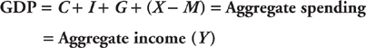
Aggregate spending (GDP) = C + I + G + (X – M)
National Income Concepts
The basic circular flow model tells us that if we add up all of the spending, it equals all of the income, and either measure provides us with GDP. This simplicity is a bit deceiving, because in practice there are several necessary accounting entries that complicate matters. We keep it simple enough for the AP exam and leave the accounting to those who wear the pocket protectors.
Aggregate Income
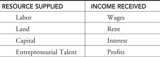
Calculating GDP from the income half of the circular flow (aka “the income approach”) must begin with incomes that are paid to the suppliers of resources. These are the households, and they supply labor, land, capital, and entrepreneurial talents. See Table 7.3 . Payments to these resources are usually referred to as wages, rents, interest, and profits. With some accounting adjustments, the sum of all income sources is approximately equal to the sum of all spending sources, or GDP.
Table 7.3
K.I.S.S.: Keep It Simple, Silly
National income accounting makes my head spin, and studying it usually sends students off to their guidance counselors to investigate majoring in Scandinavian poetry. If we focus on the simplicities of the circular flow model, we can use the relationships between income and spending with some powerful results.
• The most recent AP Macroeconomics curriculum focuses on GDP, or total spending, as the nation’s measure of economic output. Your study should therefore focus on the components of GDP.
Real and Nominal GDP
Remember that calculation of GDP requires that we take production of goods and services and apply the value of those items. But we know that prices change, so when we compare GDP from one year to the next, we have to account for changing prices. Reporting that GDP has risen without acknowledging that this is simply because prices have risen doesn’t tell a very accurate story. We need a way to compare GDP over time by accounting for different prices over time.
Example:
In 2014, our small coffee shop sold 1,000 café lattes at a price of $2 each. The total value of this production was $2,000. In 2015, firms and residents in town experienced a higher cost of living, and our coffee shop increased the price of a latte to $3 and still sold 1,000. The total value of the production has shown an increase of $1,000, but production didn’t increase at all.
Nominal GDP. The value of current production at the current prices. Valuing 2015 production with 2015 prices creates nominal GDP in 2015. This is also known as current-dollar GDP or “money” GDP.
Real GDP. The value of current production, but using prices from a fixed point in time. Valuing 2015 production at 2014 prices creates real GDP in 2015 and allows us to compare it to 2014. This is also known as constant-dollar or real GDP.
Keepin’ It Real: An Espresso Example
Suppose GDP is made up of just one product, cups of latte. Table 7.4 shows how many lattes have been made in a four-year period, the prices, and a price index. We need a price index in order to calculate real GDP. This index is a measure of the price of a good in a given year, when compared to the price of that good in a reference (or base ) year. Using 2012 as the base year, I’ll create a latte index and use it to adjust nominal GDP to real GDP for this one good. First the latte price index, or LPI:
LPI in year t = 100 × (Price of a latte in year t )/(Price of a latte in base year)
Table 7.4
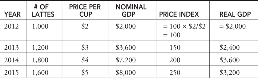
Notice that a price index always equals 100 in the base year. Even if you didn’t know the actual price of a latte in 2012, by looking at the LPI, you can see that the price doubled by 2014, since the LPI is 200 compared to the base value of 100.
Deflating Nominal GDP
To deflate a nominal value, or adjust for inflation, you do a simple division:
Real GDP = 100 × (Nominal GDP)/(Price index) or you can think of it as
Real GDP = (Nominal GDP)/(Price index; in hundreds)
Making this adjustment provides the final column of the above table. While nominal GDP appears to be rapidly rising from 2012 to 2015, you can see that, in real terms, the value of latte production has risen more modestly from 2012 to 2014 but actually fell in 2015.
Using Percentages
Another way to look at the relationship among a price index, real GDP, and nominal GDP is to look at them in terms of percentage change.
%Δ real GDP = %Δ nominal GDP – %Δ price index
Example:
If nominal GDP increased by 5 percent and the price index increased by 1 percent, we could say that real GDP increased by 4 percent.
The GDP Deflator
GDP is constructed by aggregating the consumption and production of thousands of goods and services. The prices of these many goods that compose GDP are used to construct a price index informally called the GDP price deflator. Nominal GDP is deflated, with this price index, to create real GDP. Economists watch real GDP to look for signs of economic growth and recession. We see these changes in real GDP by looking at the business cycle.
Business Cycles
The business cycle is the periodic rise and fall in economic activity, and can be measured by changes in real GDP. Figure 7.2 is a simplification of a complete business cycle. In general, there are four phases of the cycle.
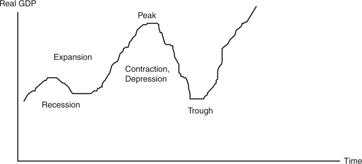
Figure 7.2
• Expansion. A period where real GDP is growing.
• Peak. The top of the cycle where an expansion has run its course and is about to turn down.
• Contraction. A period where real GDP is falling. There is no specific criteria for defining one, but a recession is unofficially described as two consecutive quarters of falling real GDP. If the contraction is prolonged or deep enough, it is called a depression.
• Trough. The bottom of the cycle where a contraction has stopped and is about to turn up.
• Though it is an imperfect measure, GDP is used as a measure of economic prosperity and growth .
• You must focus on real GDP, not nominal .
• Nominal GDP is deflated to real GDP by dividing by the price index known as the GDP deflator .
This chapter has stressed that we need to know how economic activity is measured so that we can understand how and why policies can be used to strengthen the economy. Real GDP is one of these important economic indicators and is probably the most all-encompassing of macroeconomic measures of performance, but it is not the only one. The economic indicators of inflation and unemployment are also targets of economic policy and are widely covered by the media. Before getting to macroeconomic models and policy, the next two sections spend some time learning more about what these statistics do, and do not, tell us.
7.3 Inflation and the Consumer Price Index
Main Topics: Consumer Price Index, Inflation, Is Inflation Bad?, Measurement Issues
My “Latte Price Index” illustrates that a price index can be constructed to measure changes in the price of anything. Another price index, the GDP price deflator, measures the increase in the price level of items that compose GDP. But not all goods that fall into GDP are goods that the everyday household shops for. If United Airlines buys a 767 from Boeing, it falls in GDP, but the price of a new 767 doesn’t exactly fall within what we might call consumer spending. We need a statistic that focuses on consumer prices.
The Consumer Price Index (CPI)
To measure the average price level of items that consumers actually buy, use the consumer price index (CPI). The Bureau of Labor Statistics (BLS) selects a base year, and a market basket is compiled of approximately 400 consumer goods and services bought in that year. A monthly survey is conducted in 50 urban areas around the country, and based on the results of this survey, the average prices of the items in the base year market basket is factored into the CPI. Confused yet? Let’s do a simple example of a price index for a typical consumer (see Table 7.5 ).
Table 7.5
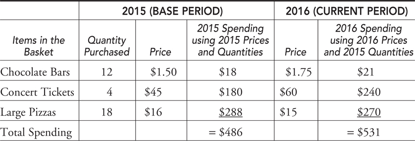
Price index current year = 100 × (Spending current year)/(Spending base year)
2016 price index = 100 × (531)/(486) = 109.26
Inflation
In the above example, the price index increased from 100 in the base year to 109.26 in 2016. In other words, the average price level increased by 9.26 percent.
On a much larger scale, the official CPI is constructed and used to measure the increase in the average price level of consumer goods. The annual rate of inflation on goods consumed by the typical consumer is the percentage change in the CPI from one year to the next.
“Know these things for multiple-choice especially.”
—Lucas, AP Student
So What Is the Difference Between the CPI and the GDP Deflator?
This concept can be confusing. The difference between these two price indices lies in the content of the market basket of goods. The CPI is based upon a market basket of goods bought by consumers, even those goods that are produced abroad. The GDP deflator includes all items that make up domestic production. Because GDP includes more than just consumer goods, the index is a broader measure of inflation, while the CPI is a measure of inflation of only consumer goods. Since consumer spending is so important to the economy, making up about 70 percent of U.S. GDP each year, the CPI is a very important indicator of what is happening in the broader economy.
• Consumer inflation rate = 100 × (CPI new – CPI old)/CPI old
• If you wished to calculate the rate of price inflation for all goods produced in a nation, you would use the GDP deflator and not the CPI .
Nominal and Real Income
As a consumer, I am also a worker and an income earner. Rising consumer prices hurt my ability to purchase the items that make me happy. In other words, rising prices can cause a decrease in my purchasing power. Ideally, I would like to see my income rise at a faster rate than the price of consumer goods. One way to see if this is happening is to deflate nominal income by the CPI to calculate my real income. Real income is calculated in the same way that real GDP is calculated.
• Real income this year = (Nominal income this year)/CPI (in hundredths)
Example:
In 2014 Kelsey’s nominal income was $40,000, and it increases to $41,000 in 2015. Curious about her purchasing power, she looks up the CPI in 2014 and finds that at the end of that year it was 234.8; at the end of 2015 it was 236.5. This is compared to the base year value of 100 in 1984.
Real income 2015 = $40,000/2.348 = $17,036
Real income 2016 = $41,000/2.365 = $17,336
What we have done here is converted Kelsey’s nominal incomes in 2014 and 2015, which were each a function of prices on those two years, into constant 1984 dollars. In other words, we have adjusted (or deflated) incomes measured in two different years so they are measured with the prices that existed in one year. After accounting for inflation, Kelsey’s real income increased by $300. Her nominal income increased at a rate slightly faster than the rate of inflation, and so her purchasing power has slightly increased.
Example:
What if Kelsey’s wages were frozen, and she did not receive that raise in 2015?
Real income 2015 = $40,000/2.365 = $16,913,
or a $123 decrease in purchasing power
Is Inflation Bad?
The previous example illustrates that inflation erodes the purchasing power of consumers if nominal wages do not keep up with prices. In general, inflation impacts different groups in different ways. It can actually help some individuals! The main thing to keep in mind with inflation is that it is the unexpected or sudden inflation that creates winners and losers. If the inflation is predictable and expected, most groups can plan for it and adjust behavior and prices accordingly.
“Make sure you understand the difference between expected and unexpected inflation.”
—AP Teacher
Expected Inflation
If my employer and I agree that the general price level is going to increase by 3 percent next year, then my salary can be adjusted by at least 3 percent so that my purchasing power does not fall. This cost of living adjustment doesn’t hurt my employer so long as the prices of the firm’s output and any other inputs also increase by 3 percent. Many unions and government employees have cost of living raises written into employment contracts to recognize predictable inflation over time.
Banks and other lenders acknowledge inflation by factoring expected inflation into interest rates. If they do not, savers and lenders can be hurt by rising prices. For this reason, the bank adds an inflation factor on the real rate of interest to create a nominal rate of interest that savers receive and borrowers pay.
Nominal interest rate = Real interest rate + Expected inflation
Savings Example 1:
When I see the bank offering an interest rate of 1 percent for a savings account and I put $100 in the bank, I expect to have $101 worth of purchasing power a year from now. But if prices increase by 2 percent, my original deposit is only worth $98. So even when I receive my $1 of interest, I have lost purchasing power.
If you have a savings account, the real rate is the rate the bank pays you to borrow your money for a year. You must be compensated for this because you do not have $100 to spend at the mall if you put it into the bank. Look at my savings example again with an inflation expectation of 2 percent and a real interest rate of 1 percent.
Savings Example 2:
• January 1: The purchasing power of my $100 is $100, and the bank offers me a 3 percent nominal interest rate on a savings account.
• Throughout the year, inflation is indeed 2 percent.
• December 31: My bank balance says $103, but $2 of purchasing power on my original deposit has been lost to inflation, leaving me with $1 as payment from the bank for having my money for one year.
Borrowing Example:
If you are looking for a loan of $100, the real interest is the rate the bank will charge you for borrowing the bank’s money for a year. After all, if the bank lends the money to you, it will not have those funds for some other profitable opportunity. Again, let’s assume that the expected inflation is 2 percent but the real rate of interest is 3 percent.
• January 1: The purchasing power of the bank’s $100 is $100, and the bank lends it to me with a 5 percent nominal interest rate.
• Throughout the year, inflation is indeed 2 percent.
• December 31: I pay the bank back $105, but $2 of the bank’s purchasing power on the original $100 has been lost to inflation, leaving it with $3 as payment from me for having its money for one year.
• So long as the actual inflation is identical to the expected inflation, workers, employers, savers, lenders, and borrowers are not harmed by the inflation.
Unexpected Inflation
When price levels are unpredictable or increase by a much larger or much smaller amount than predicted, some sectors of the economy gain and others lose. Though not a comprehensive list, some of the groups that win and lose from unexpected inflation include the following:
• Employees and employers . If the real income of workers is falling because of rapid inflation, it is possible that firms are benefiting at the expense of the workers. In a simple case, you work at a grocery store and the price of groceries unexpectedly rises by 10 percent a year, but your nominal wages rise by 8 percent. Your employer is clearly benefiting by selling goods at higher and higher prices but paying you wages that are rising more slowly.
• Fixed income recipients . A retiree receiving a fixed pension can expect to see it slowly eroded by rising prices. Likewise, a landlord who is locked into a long-term lease receives payments that slowly decline in purchasing power. If the minimum wage is not adjusted for inflation, then minimum-wage workers see a decline in their purchasing power.
• Savers and borrowers . If I put my money in the bank and leave it for a year when inflation is higher than expected, and then withdraw it, the purchasing power is greatly diminished. On the other hand, if I borrow from the bank at the beginning of that year and pay it back after higher-than-expected inflation, I am giving back dollars that are not worth as much as they used to be. This benefits me and hurts the bank.
• Rapid unexpected inflation usually hurts employees if real wages are falling, as well as fixed-income recipients, savers, and lenders.
• Rapid unexpected inflation usually helps firms if real wages are falling, as well as borrowers. It might also increase the value of some assets like real estate or other properties.
Difficulties with the CPI
Like all statistical measures, we should be careful not to read too much into them and acknowledge that they all have some problematic issues.
• Consumers substitute . The market basket uses consumption patterns from the base year, which could be several years ago. As the price of goods begins to rise, we know that consumers seek substitutes. This substitution might make the base year market basket a poor representation of the current consumption pattern.
• Goods evolve . Imagine if the CPI market basket were using 1912 as a base year. The basket would include the price of buggy whips and stove pipe hats in the inflation rate. The emergence of new products (smartphones) and extinction of others (manual typewriters) is understood by firms and consumers, but the market basket must reflect this or it risks becoming irrelevant.
• Quality differences . Some price increases are the result of improvements in quality. As automakers improve safety features, luxury options, and mechanical sophistication, we should expect the price to rise. Prices that increase because the product is fundamentally better are not an indication of overall inflation. Because the Bureau of Labor Statistics (BLS) has a difficult time telling the difference between quality improvements and actual inflation, the CPI can be overstated for this reason.
If the market basket is not altered to account for the above effects, the CPI is not very accurate. The BLS reviews the market basket from time to time and updates it if necessary. Comparisons over long periods of time are not very useful, but from month to month and year to year, the CPI is a fairly useful measure of how the average price level of consumer items is changing.
7.4 Unemployment
Main Topics: Measuring the Unemployment Rate, Types of Unemployment
Whenever an economy has idle, or unemployed, resources, it is operating inside the production possibility frontier. Though unemployment can describe any idle resource, it is almost always applied to labor.
Measuring the Unemployment Rate
Is an infant unemployed? What about an 85-year-old retiree? A parent staying home with young children? Before we can calculate an unemployment rate, we must first define who is a candidate for employment. Once again, a monthly survey is conducted by the BLS, and through a series of questions, it classifies all persons in a surveyed household above the age of 16 into one of three groups: “Employed” for pay at least one hour per week, “Unemployed” but looking for work, or “Out of the Labor Force.” If a person is out of the labor force, he has chosen to not seek employment. Our retiree and stay-at-home parent of young children would fall into this category. Many students, at least those who choose not to work, also fall into this latter category.
The non-institutionalized civilian labor force (LF) is the sum of all individuals 16 years and older, not in the military or in prison, who are either currently employed (E) or unemployed (U). To be counted as one of the unemployed, you must be actively searching for work.
LF = E + U
The unemployment rate is the ratio of unemployed to the total labor force:
UR = (U/LF) × 100
Example:
Table 7.6 summarizes the 2015 and 2016 labor market in Smallville.
Table 7.6
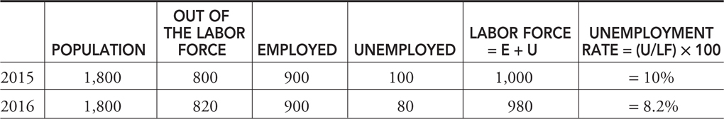
In 2015, 100 citizens are unemployed but are seeking work and the reported unemployment rate is 10 percent. After a year of searching, 20 of these unemployed citizens become tired of looking for work and move back home to live in the basement of their parents’ home. These discouraged workers are not counted in the ranks of the unemployed, and this results in an unemployment rate that falls to 8.2 percent. On the surface, the economy looks to be improving, but these 20 individuals have not found employment. The statistic hides their presence.
To give you an idea of the statistical impact that discouraged workers have on the official unemployment rate, we can look at labor force data from January 2016. The BLS estimated a U.S. labor force of 158,335,000, people and of those, 7,791,000 were counted as unemployed. The January 2016 official unemployment rate was 4.9 percent. However, there were an estimated 623,000 people who were not in the labor force because they were discouraged over their job prospects. If you add these people to the ranks of the unemployed and also to the labor force, the adjusted unemployment rate increases to 5.3 percent.
• The presence of discouraged workers understates the true unemployment rate.
“Be sure to give examples of each type.”
—AP Teacher
Types of Unemployment
People are unemployed for different reasons. Some of these reasons are predictable and relatively harmless, and others can even be beneficial to the individual and the economy. Others reasons for lost jobs are quite damaging, however, and policies need to target these types of job loss.
Frictional Unemployment . This type of unemployment occurs when someone new enters the labor market or switches jobs. Frictional unemployment can happen voluntarily if a person is seeking a better match for his or her skills, or has just finished schooling, and is usually short-lived. Employers who fire employees for poor work habits or subpar performance also contribute to the level of frictional unemployment. The provision of unemployment insurance for six months allows for a cushion to these events and assists the person in finding a job compatible with his or her skills. Because frictional unemployment is typically a short-term phenomenon, it is considered the least troublesome for the economy as a whole.
Seasonal Unemployment . This type of unemployment emerges as the periodic and predictable job loss that follows the calendar. Agricultural jobs are gained and lost as crops are grown and harvested. Teens are employed during the summers and over the holidays, but most are not employed during the school year. Summer resorts close in the winter, and winter ski lodges close in the spring. Workers and employers alike anticipate these changes in employment and plan accordingly, thus the damage is minimal. The BLS accounts for the seasonality of some employment, so such factors are not going to affect the published unemployment rate.
Structural Unemployment . This type of unemployment is caused by fundamental, underlying changes in the economy that can create job loss for skills that are no longer in demand. A worker who manually tightened bolts on the assembly line can be structurally replaced by robotics. In cases of technological unemployment like this, the job skills of the worker need to change to suit the new workplace. In some cases of structural employment, jobs are lost because the product is no longer in demand, probably because a better product has replaced it. This market evolution is inevitable, so the more flexible the skills of the workers, the less painful this kind of structural change. Government-provided job training and subsidized public universities help the structurally unemployed help themselves.
Cyclical Unemployment . Jobs are gained and lost as the business cycle improves and worsens. The unemployment rate rises when the economy is contracting, and the unemployment rate falls as the economy is expanding. This form of unemployment is usually felt throughout the economy rather than on certain subgroups, and therefore policies are going to focus on stimulating job growth throughout the economy. Structural unemployment might be forever, but cyclical unemployment only lasts as long as it takes to get through the recession.
Full Employment
Economists acknowledge that frictional and structural unemployment are always present. In fact, in a rapidly evolving economy, these are often beneficial in the long run. Because of these forms of unemployment, the unemployment rate can never be zero. Economists define full employment as the situation when there is no cyclical unemployment in the economy. The unemployment rate associated with full employment is called the natural rate of unemployment , and in the United States, this rate has traditionally been 5 to 6 percent.
![]() Review Questions
Review Questions
1 . Which of the following transactions would be counted in GDP?
(A) The cash you receive from babysitting your neighbor’s kids
(B) The sale of illegal drugs
(C) The sale of cucumbers to a pickle manufacturer
(D) The sale of a pound of tomatoes at a supermarket
(E) The eBay resale of a sweater you received from your great aunt at Christmas
2 . GDP is $10 million, consumer spending is $6 million, government spending is $3 million, exports are $2 million, and imports are $3 million. How much is spent for investments?
(A) $0 million
(B) $1 million
(C) $2 million
(D) $3 million
(E) $4 million
3 . If Real GDP = $200 billion and the price index = 200, Nominal GDP is
(A) $4 billion
(B) $400 billion
(C) $200 billion
(D) $2 billion
(E) Impossible to determine since the base year is not given
For Questions 4 to 5 use the following information for a small town:
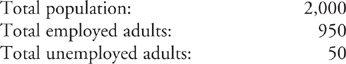
4 . What is the size of the labor force?
(A) 2,000
(B) 950
(C) 900
(D) 1,000
(E) 1,950
5 . What is the official unemployment rate?
(A) 5 percent
(B) 2.5 percent
(C) 5.5 percent
(D) 7 percent
(E) Unknown, as we do not know the number of discouraged workers
6 . You are working at a supermarket bagging groceries, but you are unhappy about your wage, so you quit and begin looking for a new job at a competing grocery store. What type of unemployment is this?
(A) Cyclical
(B) Structural
(C) Seasonal
(D) Frictional
(E) Discouraged
![]() Answers and Explanations
Answers and Explanations
1 . D —The supermarket tomatoes are the only final good sale and are counted. Babysitting is a non-market, cash “under the table” service. The sale of illegal drugs is a part of an underground economy. The sale of the cucumbers is an intermediate good. The resale of the sweater, even though it was never worn, is a second-hand sale. When your great aunt originally purchased it at the mall, it was counted in GDP.
2 . C —GDP = C + I + G + (X – M ). This would mean that 10 = 6 + I + 3 + (2 – 3); therefore, I = $2 million.
3 . B —Nominal GDP/price index (in hundredths) = Real GDP. Use this relationship to solve for Nominal GDP. $200 = (Nominal GDP)/2. Nominal GDP = $400 billion.
4 . D —Labor force is the employed + the unemployed. LF = 950 + 50 = 1,000. The remaining citizens are out of the labor force.
5 . A —The unemployment rate is the ratio of unemployed to the total labor force. UR = U/LF = 50/1,000 = 5%.
6 . D —Frictional unemployment occurs when a person is in between jobs. This person has not been laid off due to a structural change in the demand for skills, or because of a cyclical economic downturn, or because of a new season. A low wage might be discouraging; a discouraged worker is a worker who has been unemployed for so long that he or she has ceased the search for work.
![]() Rapid Review
Rapid Review
Circular flow of economic activity: A model that shows how households and firms circulate resources, goods, and incomes through the economy. This basic model is expanded to include the government and the foreign sector.
Closed economy: A model that assumes there is no foreign sector (imports and exports).
Aggregation: The process of summing the microeconomic activity of households and firms into a more macroeconomic measure of economic activity.
Gross domestic product (GDP): The market value of the final goods and services produced within a nation in a given period of time.
Final goods: Goods that are ready for their final use by consumers and firms, for example, a new Harley-Davidson motorcycle.
Intermediate goods: Goods that require further modification before they are ready for final use, e.g., steel used to produce the new Harley.
Double counting: The mistake of including the value of intermediate stages of production in GDP on top of the value of the final good.
Second-hand sales: Final goods and services that are resold. Even if they are resold many times, final goods and services are only counted once, in the year in which they were produced.
Nonmarket transactions: Household work or do-it-yourself jobs are missed by GDP accounting. The same is true of government transfer payments and purely financial transactions like the purchase of a share of IBM stock.
Underground economy: These include unreported illegal activity, bartering, or informal exchange of cash.
Aggregate spending (GDP): The sum of all spending from four sectors of the economy. GDP = C + I + G + (X – M ).
Aggregate income (AI): The sum of all income—Wages + Rents + Interest + Profit—earned by suppliers of resources in the economy. With some accounting adjustments, aggregate spending equals aggregate income.
Nominal GDP: The value of current production at the current prices. Valuing 2015 production with 2015 prices creates nominal GDP in 2015.
Real GDP: The value of current production, but using prices from a fixed point in time. Valuing 2015 production at 2014 prices creates real GDP in 2015 and allows us to compare it back to 2014.
Base year: The year that serves as a reference point for constructing a price index and comparing real values over time.
Price index: A measure of the average level of prices in a market basket for a given year, when compared to the prices in a reference (or base) year. You can interpret the price index as the current price level as a percentage of the level in the base year.
Market basket: A collection of goods and services used to represent what is consumed in the economy.
GDP price deflator: The price index that measures the average price level of the goods and services that make up GDP.
Real rate of interest: The percentage increase in purchasing power that a borrower pays a lender.
Expected (anticipated) inflation: The inflation expected in a future time period. This expected inflation is added to the real interest rate to compensate for lost purchasing power.
Nominal rate of interest: The percentage increase in money that the borrower pays the lender and is equal to the real rate plus the expected inflation.
Business cycle: The periodic rise and fall (in four phases) of economic activity.
Expansion: A period where real GDP is growing.
Peak: The top of a business cycle where an expansion has ended.
Contraction: A period where real GDP is falling.
Recession: Unofficially defined as two consecutive quarters of falling real GDP.
Trough: The bottom of the cycle where a contraction has stopped.
Depression: A prolonged, deep contraction in the business cycle.
Consumer price index (CPI): The price index that measures the average price level of the items in the base year market basket. This is the main measure of consumer inflation.
Inflation: The percentage change in the CPI from one period to the next.
Nominal income: Today’s income measured in today’s dollars. These are dollars unadjusted by inflation.
Real income: Today’s income measured in base year dollars. These inflation-adjusted dollars can be compared from year to year to determine whether purchasing power has increased or decreased.
Employed: A person is employed if she has worked for pay at least one hour per week.
Unemployed: A person is unemployed if he is not currently working but is actively seeking work.
Labor force: The sum of all individuals 16 years and older who are either currently employed (E) or unemployed (U). LF = E + U.
Out of the labor force: A person is classified as out of the labor force if he has chosen to not seek employment.
Unemployment rate: The percentage of the labor force that falls into the unemployed category. Sometimes called the jobless rate . UR = 100 × U/LF.
Discouraged workers: Citizens who have been without work for so long that they become tired of looking for work and drop out of the labor force. Because these citizens are not counted in the ranks of the unemployed, the reported unemployment rate is understated.
Frictional unemployment: A type of unemployment that occurs when someone new enters the labor market or switches jobs. This is a relatively harmless form of unemployment and not expected to last long.
Seasonal unemployment: A type of unemployment that is periodic, is predictable, and follows the calendar. Workers and employers alike anticipate these changes in employment and plan accordingly, thus the damage is minimal.
Structural unemployment: A type of unemployment that is the result of fundamental, underlying changes in the economy such that some job skills are no longer in demand.
Cyclical unemployment: A type of unemployment that rises and falls with the business cycle. This form of unemployment is felt economy-wide, which makes it the focus of macroeconomic policy.
Full employment: Exists when the economy is experiencing no cyclical unemployment.
Natural rate of unemployment: The unemployment rate associated with full employment, somewhere between 4 to 6 percent in the United States.