5 Steps to a 5: AP Macroeconomics 2017 (2016)
STEP 4
Review the Knowledge You Need to Score High
CHAPTER 8
Consumption, Saving, Investment, and the Multiplier
IN THIS CHAPTER
Summary: Having described GDP as the macroeconomic measure of a nation’s output, we begin to build a model that helps to explain how and why GDP fluctuates. As the largest component of GDP, we spend some time on consumption. Investment is also a component of GDP, but because investment plays an important role in monetary policy, we investigate it as well. The market for loanable funds combines savings and investment and is a prelude to the interaction of interest rates and the role of financial institutions. This chapter begins to show how changes in spending affect output and employment through the multiplier process. Discussion of the spending multiplier previews how policy affects the macroeconomy and leads to the aggregate demand and supply model in the next chapter.

Key Ideas
![]() Consumption and Saving Functions
Consumption and Saving Functions
![]() Investment
Investment
![]() Market for Loanable Funds
Market for Loanable Funds
![]() The Spending Multiplier, Tax Multiplier, and Balanced-Budget Multiplier
The Spending Multiplier, Tax Multiplier, and Balanced-Budget Multiplier
8.1 Consumption and Saving
Main Topics: Consumption and Saving Functions, Marginal Propensity to Consume and Save, Changes in Consumption and Saving
The circular flow model illustrates the importance of consumption in the production of goods and the employment of resources. A better understanding of consumption allows us to build a model of the macroeconomy and see the role of policy in affecting macroeconomic indicators like GDP, employment, and inflation.
Consumption and Saving Functions
Though not the only factor, the most important element affecting consumption (and savings) is disposable income. Disposable income (DI ) is what consumers have left over to spend or save once they have paid out their net taxes.
DI = Gross income – Net taxes
where Net taxes = (Taxes paid – Transfers received).
With no government transfers or taxation, DI = C + S . Though not all consumers save part of their income, typical consumers spend the majority of their disposable income and save whatever is left over. To see the relationship between disposable income and consumption, we create a consumption function .
Consumption and Saving Schedules
The consumption and saving schedules are the direct relationships between disposable income and consumption and savings. As DI increases for a typical household, C and S both increase. Table 8.1 provides an example.
Table 8.1
Consumption
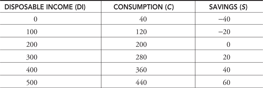
Even with zero disposable income, households still consume as they liquidate wealth (sell assets), spend some savings, or borrow (dissavings). For every additional $100 of disposable income, consumers increase their spending by $80 and increase saving by $20. We can convert the above consumption schedule to a linear equation or consumption function :
C = 40 + .80(DI)
The constant $40 is referred to as autonomous consumption because it does not change as DI changes. The slope of the consumption function is .80. This function is plotted in Figure 8.1 .
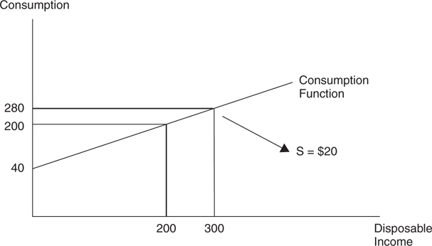
Figure 8.1
At every level of DI, the consumption function tells us how much is consumed. Both Table 8.1 and Figure 8.1 tell us that at incomes below $200, the consumer is consuming more than his income. As a result, saving is negative, and this is referred to as dissaving . But at incomes above $200, the consumer is spending less than his income, and so saving is positive.
Saving
The saving schedule above can also be converted into a linear equation, or saving function :
S = –40 + .20(DI)
The constant $–40 is referred to as autonomous saving because it does not change as DI changes. With zero disposable income, the household would need to borrow $40 to consume $40 worth of goods. The slope of the saving function is .20. This function is plotted in Figure 8.2 .
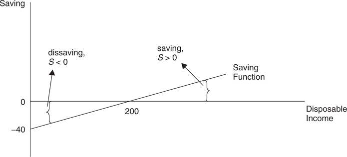
Figure 8.2
Marginal Propensity to Consume and Save
An important lesson from the study of microeconomics is the marginal concept. You can think of it in two equivalent ways. Marginal always means an incremental change caused by an external force, or it is always the slope of a “total” function. The same is true here.
The marginal propensity to consume (MPC ) is the change in consumption caused by a change in disposable income. Another way to think about it is the slope of the consumption function.
MPC = ΔC /ΔDI = Slope of consumption function
Using Table 8.1 , we see that for every additional $100 of DI, C increases by $80, so the MPC = .80.
The marginal propensity to save (MPS ) is the change in saving caused by a change in disposable income. Another way to think about it is the slope of the saving function:
MPS = ΔS /ΔDI = Slope of saving function
Using Table 8.1 , we can see that for every additional $100 of DI, S increases by $20, so the MPS = .20.
There is a nice relationship between the MPC and the MPS. For every additional dollar not consumed, it is saved. So if the consumer gains $100 in disposable income, he increases his consumption by $80 and increases saving by $20. In other words, MPC + MPS = 1. If you know one, you can find the other.

• MPC = ΔC /ΔDI = Constant slope of consumption function
• MPS = ΔS /ΔDI = Constant slope of saving function
• MPC + MPS = 1
Changes in Consumption and Saving
A change in disposable income causes a movement along the consumption and savings functions. Economists typically recognize four external determinants of household consumption and saving that shift the functions upward or downward.
Determinants of Consumption and Saving
• Wealth . When the value of accumulated wealth increases, consumption functions shift upward, and the saving function shifts downward, because households can sell stock or other assets to consume more goods at their current level of disposable income.
• Expectations . Uncertainty or a low expectation about future income usually prompts a household to decrease consumption and increase saving. An expectation of a higher future price level spurs higher consumption right now and less saving.
• Household debt . Households can increase consumption with borrowing, or debt. However, as households accumulate more and more debt, they need to use more and more disposable income to pay off the debt, and thus decrease consumption.
• Taxes and transfers . A change in taxes impacts both consumption and saving in the same direction. If the government increases taxes, households see both consumption and saving decrease because more of their gross income is sent to the government. On the other hand, an increase in government transfer payments increases both consumption and saving functions. In the case of taxes and transfers, consumption and saving functions shift in the same way.
An upward shift in consumption tells us that at all levels of disposable income, consumption is greater (C High ). If consumption is greater at all levels of disposable income, saving must be lower (S Low ), and vice versa. The only exception is the case of taxes and transfers described above. Figures 8.3 and 8.4 illustrate these simultaneous shifts in the opposite directions.
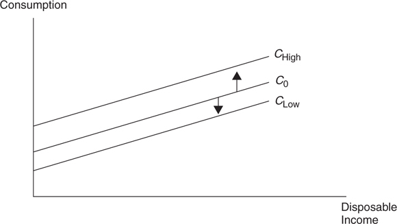
Figure 8.3
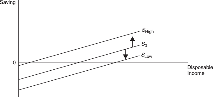
Figure 8.4
• With the exception of taxes and transfers, when the consumption function shifts upward, the saving function shifts downward.
• With the exception of taxes and transfers, when the consumption function shifts downward, the saving function shifts upward.
• When taxes increase (or transfers decrease), both consumption and saving functions shift downward.
• When taxes decrease (or transfers increase), both consumption and saving functions shift upward.
8.2 Investment
Main Topics: Decision to Invest, Investment Demand, Investment and GDP, Market for Loanable Funds
Investment is the other source of private domestic spending. We spend a little time examining why firms increase or decrease investment, build the investment demand curve, and then introduce the market for loanable funds.
Decision to Invest
The decision of a firm to spend money on new machinery or construction is simply a decision based upon marginal benefits and marginal costs. The marginal benefit of an investment is the expected real rate of return (r ) the firm anticipates receiving on the expenditure. The marginal cost of the investment is the real rate of interest (i ), or the cost of borrowing. Let’s look at this concept with examples.
Expected Real Rate of Return
A local pizza firm invests $10,000 in a new delivery car. The owner expects this to help to deliver more pizzas, increasing revenues and profits. The car lasts exactly one year and the increased real profits are anticipated to be $2,000. This expected real rate of return is $2,000/$10,000 = .20 or 20 percent. Of course an actual car lasts more than one year, but this decision to invest is shown for one year to keep it simple, while still making the point.
Real Rate of Interest
The owner goes to the bank and asks for a one-year loan to purchase the new delivery car. The bank offers a nominal rate of interest of 15 percent; this includes 5 percent for expected inflation and 10 percent as the real rate of borrowing the money for a year. At the end of the year, he spends $1,000 as real interest on the $10,000 loan.
The Decision
Since the new delivery car provides $2,000 in additional real profits (r = 20%), and the loan costs $1,000 in real interest (i = 10%), this investment should be made. Another way to make this decision is with a comparison of interest rates.
• If r % ≥ i %, make the investment.
• If r % < i %, do not make the investment.
Investment Demand
Like any demand curve, the quantity demanded increases as the price falls. The same is true for investment demand. The rational firm invests in all projects up to the point where the real rate of interest equals the expected real rate of return (i = r ). Very few investment projects are available at extremely high rates of return and so those opportunities are taken first. As the real rate of return (r ) falls, those very profitable opportunities are gone, but many less profitable investments remain. So as the expected real rate falls, the cumulative amount of investment dollars rises. Likewise, as the real cost of borrowing (i ) falls, more and more projects become worthwhile, so dollars of investment rises. Either way, as interest rates fall, the total amount of investment rises. Figure 8.5 illustrates the investment demand curve , which shows the inverse relationship between the interest rate and the cumulative dollars invested. At an interest rate of 5 percent, $20 billion dollars might be invested.
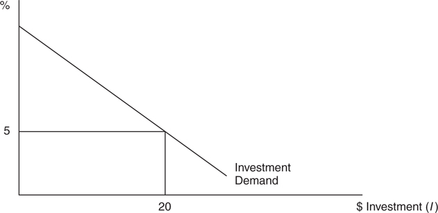
Figure 8.5
Investment and GDP
In the simple model of private investment outlined in Figure 8.5 , there is no mention of GDP or disposable income. With no government or foreign sector, GDP = DI. To keep the model simple, we assume that investment spending (I ) is determined from the investment demand curve and is constant at all levels of GDP.
Example:
In Figure 8.5 if the interest rate was 5%, firms would invest $20 billion this year, regardless of the level of disposable income or GDP. This autonomous investment is illustrated in Figure 8.6 as a horizontal line with GDP on the x axis. If something happened to interest rates, or to investment demand, autonomous investment could increase or decrease, but at that new level, would once again be constant at any value of GDP.
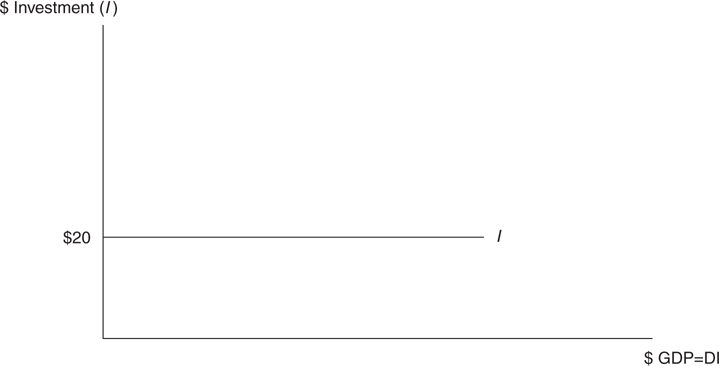
Figure 8.6
Market for Loanable Funds
It is useful to see the relationship between saving and investment by looking at the market for loanable funds. When savers place their money in banks or buy bonds, those funds are available to be borrowed by firms for private investment.
Demand for Loanable Funds
The inverse relationship between investment and the real interest rate is fairly straightforward. As the real interest rate falls, borrowing becomes less costly, and large investment projects become more attractive to firms. This investment demand curve can also be thought of as a demand for loanable funds, and this demand is the result of the borrowing by private firms and the government.
Supply of Loanable Funds
The supply of loanable funds comes from saving on the part of households, both domestic and foreign. If disposable income is greater than consumption, this private saving exists, and is positively related to the real interest rate.
The market for loanable funds is shown in Figure 8.7 , and the equilibrium interest rate is found at the intersection of the supply and demand curves. In upcoming chapters, we investigate the role of this market in the banking system, fiscal and monetary policy, and economic growth.
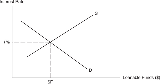
Figure 8.7
“Make the connections between concepts learned in a previous chapter to what you are learning now, because everything is cumulative.”
—Caroline, AP Student
• The supply of loanable funds comes from saving, and lending.
• The demand for loanable funds comes from investment, and borrowing.
• Equilibrium is at the real interest rate where dollars saved equals dollars invested.
8.3 The Multiplier Effect
Main Topics: Multiplier Effect and Spending Multiplier, Public and Foreign Sectors, Tax Multiplier, Balanced-Budget Multiplier
The most simple circular flow consists solely of consumers and firms; in other words, GDP = C + I . But the public sector (G ) and foreign sector (X – M ) are also important sources of domestic spending and income. Inclusion of these two sectors provides very little in the way of complications; they introduce the concept of the spending multiplier, the tax multiplier, and the balanced budget multiplier. This also paves the way for fiscal policy aimed at macroeconomic stability.
Multiplier Effect and Spending Multiplier
When you buy an ear of corn at the farmers’ market, those dollars serve as income to several people. The farmers use those dollars to pay employees, to run their farm equipment, and to buy their own food. Farm employees use those wages to buy bacon, pay the rent, and many other goods and services. The circular flow explains how the injection of a few dollars of spending creates many more dollars of spending. Follow the dollars for a few rounds to see how it works. With the marginal propensity to consume of .80, if households receive a $1 of new income they spend $.80 and save $.20.
Round 1: Firms increase investment spending by $10 , which acts as an injection of new money into the economy.
Round 2: The $10 acts as income to resource suppliers (households) and with an MPC = .80, households spend $8 and save $2.
Round 3: The $8 of new consumption spending (C ) is income for other households, and they also spend 80 percent, or $6.40 and save $1.60.
Round 4: The $6.40 of new C is income for other households, and they spend 80 percent, or $5.12 , and save $1.28.
This process repeats. Each time the dollars circulate through the economy, 80 percent is spent and 20 percent is saved. After only four rounds, there has been $10 + 8 + 6.40 + 5.12 = $29.52 of new GDP . The process continues until households are trying to consume 80 percent of virtually nothing and the increase in new GDP comes to an eventual stop.
This is called the multiplier effect . A change in any component of autonomous spending creates a larger change in GDP. The discussion of the “rounds” of spending above implies that the marginal propensities to consume and save play a critical role in determining the magnitude of the multiplier. There are two equivalent ways to calculate the multiplier if you know the MPC or MPS. The magnitude of the spending multiplier is found by taking a ratio:
Multiplier = 1/(1 – MPC) = 1/ (1 – .80) = 5
Since MPC + MPS = 1,
Multiplier = 1/ MPS = 1/.20 = 5.
The spending multiplier can be found by using one of the following equations:
• Multiplier = 1/MPS
• Multiplier = 1/(1–MPC)
• Multiplier = (Δ GDP)/(Δ Spending)
Some common spending multipliers are as follows:
• MPC = .90, Multiplier = 1/.10 = 10
• MPC = .80, Multiplier = 1/.20 = 5
• MPC = .75, Multiplier = 1/.25 = 4
• MPC = .50, Multiplier = 1/.5 = 2
Public and Foreign Sectors
The inclusion of government spending (G ) and net exports (X – M ) act in the very same way as the change in investment illustrated in the preceding example.
Government Spending (G )
With the MPC =.80, we have found the spending multiplier equal to 5. If autonomous government spending is incorporated into the circular flow model, the multiplier effect is again felt throughout the economy. If G = $20, we could expect those $20 to multiply to $100 in new GDP.
Net Exports (X –M )
The final sector of the macroeconomy is the foreign sector. The addition or subtraction (if imports exceed exports) of autonomous net exports is an increase (or decrease) of dollars in the circular flow. Using a spending multiplier of 5, if (X – M ) = $10, GDP would increase by $50.
Tax Multiplier
The preceding discussion of the public sector shows that when the government injects money into the economy (G ), it multiplies by a factor of the spending multiplier. But the government can also have an impact on aggregate expenditures and real GDP by changing taxes and/or transfers.
The Multiplier Effect
Recipients of a decrease in taxes treat it as an increase in disposable income. The typical household increases consumption by a factor of the MPC and increases saving by a factor of the MPS. It is important to keep in mind that less than 100 percent of this increase in disposable income circulates through the economy because most households save a proportion of it.
Example:
The MPC is equal to .90, and the government transfers back tax revenue to consumers by sending each taxpayer a $200 check. With an MPC = .90, $180 is consumed and $20 is saved. The multiplier process kicks in, but not on the entire $200, only on the consumed portion of $180. The multiplier being 1/.10 = 10, GDP increases by $1,800.
In other words, a $200 change in tax policy (a tax rebate in this case) caused an $1,800 change in real GDP. This tax multiplier of 9 measures the magnitude of the multiplier process when there is a change in taxes.
“Remember that taxes will have a smaller multiplier than government spending!”
—Richard, AP Student
The Difference in Multipliers
With an MPC = .90, the spending multiplier is 10, but the tax multiplier is smaller, Tm = 9. Why? The spending multiplier begins to work as soon as there is a change in autonomous spending (C, I, G , net exports), but the tax multiplier must first go through a person’s consumption function as disposable income. In that first “round” of spending, some of those injected dollars are leakages in the form of savings. In the example above, 10 percent of those injected dollars fail to be recirculated, and therefore the final multiplier effect is smaller. The relationship between the spending multiplier and the tax multiplier (Tm) is as follows:
Tm = MPC × (Spending multiplier) = .90 × (l/.10) = 9 in our example
Be prepared to respond to a free-response question that asks you to explain why the tax multiplier is smaller than the spending multiplier.
Example:
The MPC = .80 and the government decides to impose a $50 increase in taxes. What happens to GDP?
Tm = .80 × Multiplier = .80 × (1/.20) = 4
Because the tax multiplier is equal to 4, we determine that GDP falls by $200. How do we know? Because taxes were increased , disposable income falls, consumption falls, causing GDP to fall, in this case by a factor of 4.
The tax multiplier is found by:
• Tm = (Δ GDP)/(Δ taxes)
• Tm = MPC × M = MPC/MPS
Balanced-Budget Multiplier
The government both collects and spends tax revenue. In a simplified model, if the dollars spent equal the dollars collected, the budget is balanced. We have already discussed how the spending multiplier and tax multiplier are different. A quick example of a balanced budget policy illustrates what is called the balanced-budget multiplier.
Example:
The government wants to spend $100 on a federal program and pay for it by collecting $100 in additional taxes. The MPC = .90 in this example.
Spending Effect
The spending multiplier = 10 implies that the $100 of new spending (G ) creates a $1,000 increase in real GDP.
Taxation Effect
The tax multiplier Tm = 9 implies that a $100 increase in taxes decreases real GDP by $900.
Balanced Budget Effect
Change in real GDP = +$1,000 – $900 = +$100
So a $100 increase in spending, financed by a $100 increase in taxes, created only $100 in new GDP. The balanced-budget multiplier is always equal to 1, regardless of the MPC .
• Balanced-budget multiplier = 1
![]() Review Questions
Review Questions
1 . When disposable income increases by $X ,
(A) consumption increases by more than $X .
(B) saving increases by less than $X .
(C) saving increases by exactly $X .
(D) saving remains constant.
(E) saving decreases by more than $X .
2 . Which of the following is true about the consumption function?
(A) The slope is equal to the MPC.
(B) The slope is equal to the MPS.
(C) The slope is equal to MPC + MPS.
(D) It shifts upward when consumers are more pessimistic about the future.
(E) It shifts downward when consumer wealth increases in value.
3 . Which of the following events most likely increases real GDP?
(A) An increase in the real rate of interest
(B) An increase in taxes
(C) A decrease in net exports
(D) An increase in government spending
(E) A lower value of consumer wealth
4 . Which of the following choices is most likely to create the greatest decrease in real GDP?
(A) The government decreases spending, matched with a decrease in taxes.
(B) The government increases spending with no increase in taxes.
(C) The government decreases spending with no change in taxes.
(D) The government holds spending constant while increasing taxes.
(E) The government increases spending, matched with an increase in taxes.
5 . The tax multiplier increases in magnitude when
(A) the MPS increases.
(B) the spending multiplier falls.
(C) the MPC increases.
(D) government spending increases.
(E) taxes increase.
6 . Which of the following is the source of the supply of loanable funds?
(A) The stock market
(B) Investors
(C) Net exports
(D) Banks and mutual funds
(E) Savers
![]() Answers and Explanations
Answers and Explanations
1 . B —A $1 increase in DI increases consumption by a factor of the MPC and increases saving by a factor of the MPS. Because both MPC and MPS represent the fraction of new income that is consumed and saved, consumption and saving increase by less than the increase in DI.
2 . A —The slope of the consumption function is the MPC. The slope of the saving function is the MPS.
3 . D —An increase in GDP is the result of an increase in C, I, G , or (X – M ). All other choices represent less spending in some economic sector.
4 . C —Look for choices that decrease GDP by the largest magnitude. Choices B and E actually improve the economy (and GDP), so they are eliminated. A decrease in spending lowers GDP by a magnitude equal to the spending multiplier, which is larger than the tax multiplier, which in turn is larger than the balanced budget multiplier. This question is a prelude to fiscal policy.
5 . C —Knowing the relationship between the tax and spending multipliers allows you to make the right choice. Tm = MPC × Multiplier = MPC/MPS.
6 . E —Banks help facilitate lending to investors, but the real supply of those loanable funds are the savers who choose to place some of their disposable income dollars in those banks as saving.
![]() Rapid Review
Rapid Review
Disposable income (DI): The income a consumer has left over to spend or save once he or she has paid out net taxes. DI = Y – T .
Consumption and saving schedules: Tables that show the direct relationships between disposable income and consumption and saving. As DI increases for a typical household, C and S both increase.
Consumption function: A linear relationship showing how increases in disposable income cause increases in consumption.
Autonomous consumption: The amount of consumption that occurs no matter the level of disposable income. In a linear consumption function, this shows up as a constant and graphically it appears as the y intercept.
Saving function: A linear relationship showing how increases in disposable income cause increases in saving.
Dissaving: Another way of saying that saving is less than zero. This can occur at low levels of disposable income when the consumer must liquidate assets or borrow to maintain consumption.
Autonomous saving: The amount of saving that occurs no matter the level of disposable income. In a linear saving function, this shows up as a constant and graphically it appears as the y intercept.
Marginal Propensity to Consume (MPC): The change in consumption caused by a change in disposable income, or the slope of the consumption function: MPC = ΔC /ΔDI.
Marginal propensity to save (MPS): The change in saving caused by a change in disposable income, or the slope of the saving function: MPS = ΔS /ΔDI.
Determinants of consumption and saving: Factors that shift the consumption and saving functions in the opposite direction are wealth, expectations, and household debt. The factors that change consumption and saving functions in the same direction are taxes and transfers.
Expected real rate of return (r): The rate of real profit the firm anticipates receiving on investment expenditures. This is the marginal benefit of an investment project.
Real rate of interest (i): The cost of borrowing to fund an investment. This can be thought of as the marginal cost of an investment project.
Decision to invest: A firm invests in projects as long as r ≥ i .
Investment demand: The inverse relationship between the real interest rate and the cumulative dollars invested. Like any demand curve, this is drawn with a negative slope.
Autonomous investment: The level of investment determined by investment demand. It is autonomous because it is assumed to be constant at all levels of GDP.
Market for loanable funds: The market for dollars that are available to be borrowed for investment projects. Equilibrium in this market is determined at the real interest rate where the dollars saved (supply) is equal to the dollars borrowed (demand).
Demand for loanable funds: The negative relationship between the real interest rate and the dollars invested and borrowed by firms and by the government.
Private saving: Saving conducted by households and equal to the difference between disposable income and consumption.
Supply of loanable funds: The positive relationship between the dollars saved and the real interest rate.
Multiplier effect: Describes how a change in any component of aggregate expenditures creates a larger change in GDP.
Spending multiplier: The magnitude of the spending multiplier effect is calculated as = (ΔGDP)/(Δ spending) = 1/MPS = 1/(1 – MPC).
Tax multiplier: The magnitude of the effect that a change in taxes has on real GDP. Tm = (ΔGDP)/(Δ taxes) = MPC × Multiplier = MPC/MPS.
Balanced-budget multiplier: When a change in government spending is offset by a change in lump-sum taxes, real GDP changes by the amount of the change in G ; the balanced-budget multiplier is thus equal to 1.