5 Steps to a 5: AP Macroeconomics 2017 (2016)
STEP 4
Review the Knowledge You Need to Score High
CHAPTER 9
Aggregate Demand and Aggregate Supply
“This is the bulk of the Macro exam––very important!”
—AP Teacher
IN THIS CHAPTER
Summary: Chapter 7 addressed three widely used measures of macroeconomic performance: real GDP, inflation, and unemployment. Economists have built upon the models of supply and demand for microeconomic markets to model an aggregate picture of the macroeconomy. The models of Aggregate Demand (AD) and Aggregate Supply (AS) have been extremely useful to predict how real GDP, employment, and the average price level are affected by external factors and government policy. Before discussing macroeconomic policy, we first need to describe the AD/AS model.

Key Ideas
![]() Aggregate Demand (AD)
Aggregate Demand (AD)
![]() Aggregate Supply (AS)
Aggregate Supply (AS)
![]() Short-Run and Long-Run AS
Short-Run and Long-Run AS
![]() Macroeconomic Equilibrium
Macroeconomic Equilibrium
![]() The Inflation and Unemployment Trade-Off
The Inflation and Unemployment Trade-Off
9.1 Aggregate Demand (AD)
Main Topics: What Is Aggregate Demand?, Components of AD, The Shape of AD, Changes in AD
When we discussed microeconomic markets, we described the shape of any microeconomic demand curve with the Law of Demand, income, and substitution effects. Both effects work to change quantity demanded in the opposite direction of any price change. What tends to be the case for the demand of a microeconomic good is also the case for AD, but for different theoretical reasons.
What Is Aggregate Demand?
A microeconomic demand curve for peaches illustrates the relationship between the quantity of peaches demanded and the price of peaches. When economists aggregate all microeconomic markets to build AD, we include peaches and all other items that are domestically produced. Aggregate demand is the relationship between all spending on domestic output and the average price level of that output.
Components of AD
Demand in the macroeconomy comes from four general sources, and we have already seen these components when we described how total production is measured in the economy. In the previous chapter we defined real GDP as = C+ I +G + (X – M ).
So AD measures, for any price level, the sum of consumption spending by households, investment spending by firms, government purchases of goods and services, and the net exports bought by foreign consumers.
The Shape of AD
When the price of peaches rises, consumers find another microeconomic good (with a lower relative price) to substitute for peaches, and this helps explain why the demand for peaches is downward sloping. But if the overall price level is rising, the price of peaches, pears, and apples might all be rising. Remember that this average price level is not the same as the price of one good relative to another. Where are the substitutes when the “good” we are discussing is a unit of real GDP? Macroeconomists describe three general groups of substitutes for national output:
• Goods and services produced in other nations (foreign sector substitution effect)
• Goods and services in the future (interest rate effect)
• Money and financial assets (wealth effect)
Foreign Sector Substitution Effect . When the average price of United States output (as measured by the CPI or some other price index) increases, consumers naturally begin to look for similar items produced elsewhere. A Japanese computer, a German car, and a Mexican textile all begin to look more attractive when inflation heats up in the United States. The resulting increase in imports pushes real GDP down at a higher price level.
Interest Rate Effect . Remember that consumers have two general choices with their disposable income: they can consume it or they can save it for future consumption. If the average price level rises, consumers might need to borrow more money for big-ticket items like autos or college tuition. When more and more households seek loans, the real interest rate begins to rise, and this increases the cost of borrowing. Firms postpone their investment in plant and equipment, and households postpone their consumption of more expensive items for a future when their spending might go further and borrowing might be more affordable. This wait-and-see mentality reduces current consumption of domestic production as the price level rises and real GDP falls.
Wealth Effect . Wealth is the value of accumulated assets like stocks, bonds, savings, and especially cash on hand. As the average price level rises, the purchasing power of wealth and savings begins to fall. Higher prices therefore tend to reduce the quantity of domestic output purchased.
The combination of the foreign sector substitution, interest rate, and wealth effects predict a downward-sloping AD curve. For all three reasons, as the overall price level rises, consumption of domestic output (real GDP) falls along the AD curve. This is seen as a movement from points a to b in Figure 9.1 .
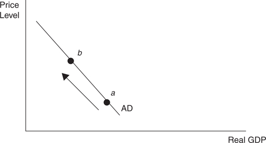
Figure 9.1
• Aggregate demand is not the vertical or horizontal summation of the demand curves for all microeconomic goods and services.
• AD is a model of how domestic purchasing changes when the aggregate price level changes.
Changes in AD
Since AD is the sum of the four components of domestic spending [C, I, G , (X – M )], if any of these components increases, holding the price level constant, AD increases, which increases real GDP. This is seen as a shift to the right of AD. If any of these components decreases, holding the price level constant, AD decreases, which decreases real GDP. This is seen as a shift to the left of AD. Figure 9.2 illustrates these shifts in AD.
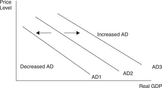
Figure 9.2
This is a preview for policy to manipulate the macroeconomy. If you want to stimulate real GDP and lower unemployment, you need to boost any or all of the components of AD. If you feel AD must slow down, you need to rein in the components of AD. Policies are tackled in more depth in the next chapter, but for now we’ll take a quick look at some variables that can increase C, I, G , or (X – M ).
Consumer Spending (C ). If you put more money in the pockets of households, expect them to consume a great deal of it and save the rest. Consumers also increase their consumption if they are more optimistic about the future.
Investment Spending (I ). Firms increase investment if they believe the investment will be profitable. This expected return on the investment is increased if investors are optimistic about the future profitability, or if the necessary borrowing can be done at a low rate of interest.
Government Spending (G ). The government injects money into the economy by spending more on goods and services, by reducing taxes, or by increasing transfer payments.
1. Government spending on goods and services acts as a direct increase in AD.
2. Taxes and transfers . Lowering taxes and increasing transfer payments increase AD through C by increasing DI.
Net Exports (X – M ). When we sell more goods to foreign consumers and buy fewer goods from foreign producers, this component of AD increases.
1. Foreign incomes . Exports (X ) increase with a strong Canadian, Mexican, or Brazilian economy. When foreign consumers have more disposable income, this increases the AD in the United States because those consumers spend some of that income on U.S.-made goods.
2. Consumer tastes . Consumer tastes and preferences, both foreign and domestic, are constantly changing. If American blue jeans become more popular in France, American AD increases. If French wines become more preferred by American consumers, AD in France increases.
3. Exchange rates . Imports (M ) decrease when the exchange rate between the U.S. dollar and foreign currency falls. The model of foreign currency exchange is covered in a later chapter, but the idea is that foreign goods become relatively more expensive and so domestic consumers buy fewer foreign-produced items.
9.2 Aggregate Supply (AS)
Main Topics: What Is Aggregate Supply?, Short-Run and Long-Run Shape of AS, Changes in AS
Again, there are parallels between our coverage of supply in micro markets and aggregate supply. The law of supply describes the positive relationship between the micro price of a product and the quantity of that product that firms supply, and is explained in part by increasing marginal cost as output rises. What tends to be the case for the supply of a micro good is also the case for AS, but for different theoretical reasons.
What Is Aggregate Supply?
A microeconomic supply curve for salt illustrates the relationship between the price of salt and the quantity of salt supplied. When economists aggregate all microeconomic markets to build AS, we include salt and all other items that are domestically supplied. Aggregate supply is the relationship between the average price level of all domestic output and the level of domestic output produced.
Short-Run and Long-Run Shape of AS
The model of AS and the resulting shape of the AS curve depend upon whether the economy has fully adjusted to market forces and price changes.
Macroeconomic Short Run
In the macroeconomic short run period of time, the prices of goods and services are changing in their respective markets, but input prices have not yet adjusted to those product market changes. This lag between the increase in the output price and the increase in input prices gives us a shape of the short-run AS curve that is described in three stages. Figure 9.3 illustrates the stages of short-run AS.
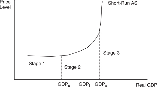
Figure 9.3
If the economy is in a recession with low production (GDPu ), there are many unemployed resources. Increasing output from this low level puts little pressure on input costs and subsequent minimal increase in the overall price level. The first stage of AS is drawn as almost horizontal. The Keynesian school of economics believes that when aggregate spending is extremely weak, the economy can be modeled in this way.
As real GDP increases in the second stage of AS and approaches full employment (GDPf ), available resources become more difficult to find, and so input costs begin to rise. If the price level for output rises at a faster rate than the rising costs, producers have a profit incentive to increase output. Most of the time the economy is operating in this upward-sloping range of AS, and so you see short-run AS commonly drawn with a positive slope.
If the economy grows and approaches the nation’s productive capacity (GDPc ), firms cannot find unemployed inputs. Input costs and the price level rise much more sharply, and so in this third stage of AS, the curve is almost vertical.
Macroeconomic Long Run
The period of time known as the macroeconomic long run is long enough for input prices to have fully adjusted to market forces. Now all product and input markets are in equilibrium, and the economy is at full employment. In this long-run equilibrium, the AS curve is vertical at GDPf . The Classical school of economics asserts that the economy always gravitates toward full employment; so a cornerstone of classical macroeconomics is a vertical AS curve. Figure 9.4 illustrates the long-run AS curve.
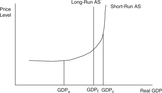
Figure 9.4

• When drawing the AD/AS graph for a free-response question, it is not acceptable to label the vertical axis “P” or “$” and the horizontal axis “Q.” You want to be very careful to use terms like “Aggregate price level” or “PL” on the vertical axis and “Real output” or “Real GDP” on the horizontal axis to earn these graphing points.
Changes in AS
In the short run, AS may fluctuate without changing the level of full employment. There are some factors, however, that can cause a fundamental shift in the long-run AS curve because they can change the level of output at full employment.
Short-Run Shifts
The most common factor that affects short-run AS is an economy-wide change in input (or factor) prices. Taxes, government policy, and short-term political or natural events can change the short-term ability of a nation to supply goods and services.
• Input prices . If input prices fall, the short-run AS curve increases (shifting to the right) without changing the level of full employment.
• Tax policy . Some taxes are aimed at producers rather than consumers. If these “supply-side taxes” are lowered, short-run AS shifts to the right.
• Deregulation . In some cases, the regulation of industries can restrict their ability to produce (for good reasons in many cases). If these regulations are lessened, the short-run AS likely increases.
• Political or environmental phenomena . For a nation as large as the United States, wars and natural disasters can decrease the short-run AS without permanently decreasing the level of full employment. For a smaller nation or a large nation hit by an epic disaster, this could be a permanent decrease in the ability to produce.
Long-Run Shifts
There are a few main factors that affect both long-run and short-run AS and fundamentally affect the level of full employment in a nation’s macroeconomy:
• Availability of resources . A larger labor force, larger stock of capital, or more widely available natural resources can increase the level of full employment.
• Technology and productivity . Better technology raises the productivity of both capital and labor. A more highly trained or educated populace increases the productivity of the labor force. These factors increase long-run AS over time.
• Policy incentives . Different national policies like unemployment insurance provide incentives for a nation’s labor force to work. If policy provides large incentives to quickly find a job, full-employment real GDP rises. If government gives tax incentives to invest in capital or technology, GDPf rises.
Example:
In the 1990s, the U.S. economy saw dramatic increases in technology and investment in the capital stock. This period produced a significant increase in the real GDP at full employment, as shown in Figure 9.5 .
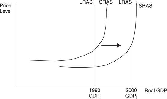
Figure 9.5
• When the LRAS curve shifts to the right, this indicates economic growth, just as an outward shift in the production possibility curve does.
9.3 Macroeconomic Equilibrium
Main Topics: Equilibrium Real GDP and Price Level, Recessionary and Inflationary Gaps, Shifting AD, The Multiplier Again, Shifting SRAS, Classical Adjustment from Short-Run to Long-Run Equilibrium
We use supply and demand models to predict changes in the prices and quantities of microeconomic goods and services. Now that we have built a model of aggregate demand and aggregate supply, we use similar analysis to predict changes in real GDP and the average price level.
Equilibrium Real GDP and Price Level
When the quantity of real output demanded is equal to the quantity of real output supplied, the macroeconomy is said to be in equilibrium. Figure 9.6 illustrates macroeconomic equilibrium at full employment Q f and price level PLf at the intersection of AD, SRAS, and LRAS.
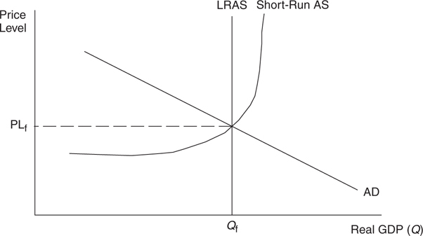
Figure 9.6
Recessionary and Inflationary Gaps
When the economy is in equilibrium, but not at the level of GDP that corresponds to full employment (GDPf ), the economy is experiencing either a recessionary or an inflationary gap. As the name implies, a recessionary gap exists when the economy is operating below Q f and the economy is likely experiencing a high unemployment rate. In Figure 9.7 , the recessionary gap is the difference between GDPf and GDPr , or the amount that GDP must rise to reach GDPf .
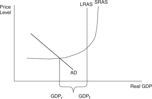
Figure 9.7
An inflationary gap exists when the economy is operating above GDPf . Because production is higher than GDPf , a rising price level is the greatest danger to the economy. In Figure 9.8 , the inflationary gap is the difference between GDPi and GDPf , or the amount that GDP must fall to reach GDPf .
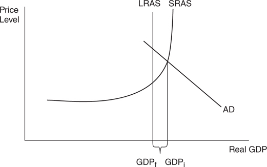
Figure 9.8
“Be able to locate these on a graph.”
—AP teacher
Shifting AD
Since you have mastered the microeconomic tools of supply and demand, you should have little trouble predicting how macroeconomic factors affect real GDP and the price level.
Shifts in AD
The economy is currently in equilibrium but at a very low recessionary level of real GDP. If AD increases from AD0 to AD1 in the nearly horizontal range of SRAS, the price level may only slightly increase, while real GDP significantly increases and the unemployment rate falls.
If AD continues to increase to AD2 in the upward-sloping range of SRAS, the price level begins to rise and inflation is felt in the economy. This demand-pull inflation is the result of rising consumption from all sectors of AD.
If AD increases much beyond full employment to AD3 , inflation is quite significant and real GDP experiences minimal increases. Figures 9.9 , 9.10 , and 9.11 illustrate how rising AD has different effects on the price level and real GDP in the three stages of short-run AS.
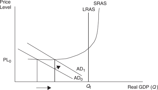
Figure 9.9
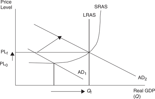
Figure 9.10
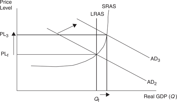
Figure 9.11
If aggregate demand weakens, we can expect the opposite effects on price level and real GDP. In fact, one of the most common causes of a recession is falling AD as it lowers real GDP and increases the unemployment rate. Inflation is not typically a problem with this kind of recession, as we expect the price level to fall, or deflation , with a severe decrease in AD. This is seen in Figure 9.12 .
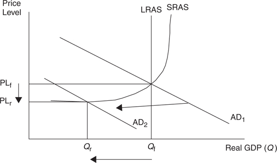
Figure 9.12
The Multiplier Again
One of the important topics of the previous chapter is the spending multiplier. When a component of autonomous spending increases by $1, real GDP increases by a magnitude of the multiplier. The full multiplier effect is only observed if the price level does not increase, and this only occurs if the economy is operating on the horizontal range of the SRAS curve. Figure 9.13 shows the full multiplier effect. (Note that the SRAS curve is likely a much smoother curve, but the multiplier effect can be illustrated more clearly with more linear segments.)
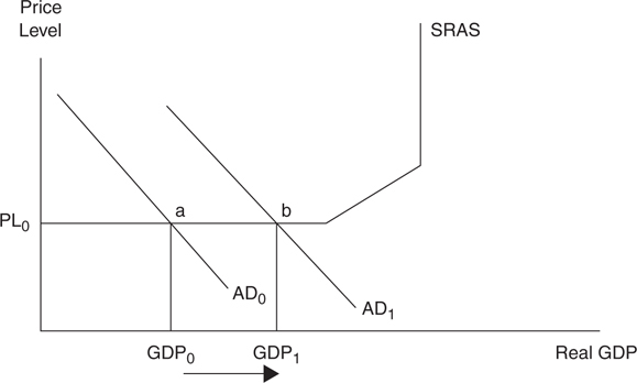
Figure 9.13
But what if the economy is operating in the upward-sloping range of SRAS? Figure 9.14 shows an identical rightward shift in AD. If there were no increase in the price level, the new equilibrium GDP would be at GDP1 , but with a rising price level, it is somewhat smaller at GDP2 . This means that the full multiplier effect is not felt because the rising price level weakens the impact of increased spending in the macroeconomy.
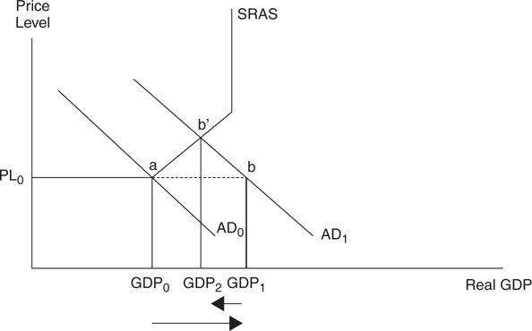
Figure 9.14
• The multiplier effect of an increase in AD is greater if there is no increase in the price level.
• The multiplier effect of an increase in AD is smaller if there is a larger increase in the price level.
Shifting SRAS
The macroeconomy is currently in equilibrium at full employment. In Figure 9.15 , we simplify the short-run aggregate supply curve by drawing only the upward-sloping segment (and this is the usual treatment of SRAS in the AP curriculum). If nominal input prices were to fall, the SRAS curve shifts to the right. Assuming that the AD curve stays constant, the price level falls, real GDP increases, and the unemployment rate falls. This kind of supply-side boom would seemingly be the best of all situations, though it is likely to only be temporary. When the economy is producing beyond Q f, eventually the high demand for production inputs will increase the prices of those inputs, shifting the SRAS curve back to the left and returning the economy to full employment.
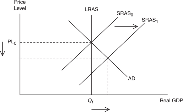
Figure 9.15
If an increase in SRAS is the best of possible macroeconomic situations, a decrease in SRAS is one of the worst. Figure 9.16 shows that a decrease, or leftward shift, in SRAS creates inflation, lowers real GDP, and increases the unemployment rate. This cost-push inflation , or stagflation , creates very unpleasant economic conditions in the short run. In the long run, however, the high unemployment should eventually relieve pressure on nominal input prices. When the input prices begin to fall, the SRAS shifts back to the right, returning the economy to full employment.
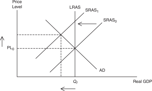
Figure 9.16
“Make it easier for the graders and use flow charts to answer free-response questions instead of long essays.”
—Justine, AP Student
Supply Shocks
These shifts in SRAS are caused by events that are called supply shocks . A supply shock is an economy-wide phenomenon that affects the costs of firms, positively or negatively. Positive supply shocks might be the result of higher productivity or lower energy prices. Negative supply shocks usually occur when economy-wide input prices suddenly increase, like the OPEC oil embargoes of the 1970s or the Gulf War of 1990 to 1991.
• ↑ AD causes ↑ real GDP, ↓ unemployment and ↑ price level.
• ↓ AD causes ↓ real GDP, ↑ unemployment and ↓ price level.
• ↑ SRAS causes ↑ real GDP, ↓ unemployment and ↓ price level.
• ↓ SRAS causes ↓ real GDP, ↑ unemployment and ↑ price level.
Classical Adjustment from Short-Run to Long-Run Equilibrium
One of the toughest concepts for students to master is the way in which the AD/AS model presents both a short-run and a long-run equilibrium. Although some economists disagree, the prevailing treatment in the AP curriculum is that a recessionary or inflationary gap (a short-run equilibrium) will “self-correct” to a long-run equilibrium once enough time has passed for all prices to adjust. Let’s see how this can happen.
Adjustment to a Recessionary Gap
Suppose the economy is currently operating at full employment, as shown in Figure 9.17 at the intersection of the AD, SRAS, and LRAS curves with a real GDP of Q f . Now suppose that consumers and firms begin to lose confidence in the labor market and overall economy, causing AD to shift to the left. In the short run, this will cause a recessionary gap as real GDP falls to Q r (unemployment rises), and the aggregate price level falls from PL1 to PL2. Ignoring any kind of fiscal or monetary policy intervention (which we will discuss in the next two chapters), this short-run recessionary gap can self-correct. How does this happen?
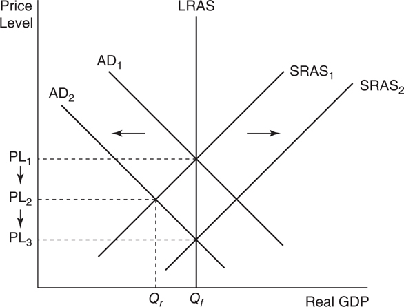
Figure 9.17
One of the hallmarks of a recession is a decreased demand for many factors of production, like labor, steel, oil, and other commodities. This decreased demand for critical factors of production will eventually decrease the prices of those factors, causing a gradual rightward shift of the SRAS curve to SRAS2 . The SRAS curve shifts to the right until the recessionary gap is closed, the economy is back at Q f , and an even lower aggregate price level exists at PL3 .
Adjustment to an Inflationary Gap
Let’s begin again with long-run equilibrium at a real GDP of Q f . When we incorporate an increase in the AD curve, we create an inflationary gap. Figure 9.18 shows that this increase to AD2 causes an increase in real GDP to Q i (a lower unemployment rate) and an increase in the aggregate price level to PL2 . How would this self-correct?
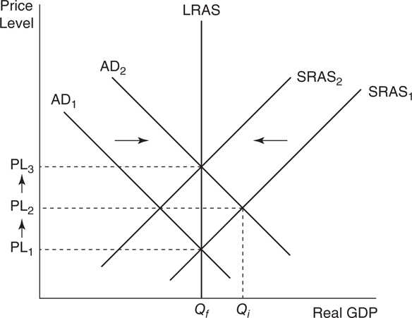
Figure 9.18
When the economy is really booming, there is stronger demand for labor and all of those other factors of production, and this causes factor prices to rise. As the factor prices rise, the SRAS curve begins to shift to the left to SRAS2 . Eventually, the inflationary gap is eliminated, and the economy is back in long-run equilibrium at Q f , though at an even higher aggregate price level of PL3 .
• Using the AD/AS model to show the long-run adjustment to equilibrium after a short-run shift in AD is a very common FRQ on the AP Macroeconomics exam.
9.4 The Trade-Off Between Inflation and Unemployment
Main Topics: Short-Run Changes in AD, The Phillips Curve, The Long-Run Phillips Curve, Expectations
Changes in AD and AS create changes in our main macroeconomic indicators of inflation and unemployment. Many economists have studied the relationship between inflation and unemployment, and this section provides a very brief overview of one prominent theory, the Phillips curve. We also take another look at the effects of supply shocks and expectations.
Short-Run Changes in AD
In the upward-sloping range of the SRAS curve, there is a positive relationship between the price level and output. If AD is rising, the price level and real GDP are both rising. Since rising real GDP creates jobs and lowers unemployment, we connect these points of equilibrium and show an inverse relationship between inflation and the unemployment rate. See Figure 9.19 .
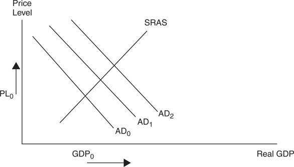
Figure 9.19
The Phillips Curve
The inverse relationship between inflation and the unemployment rate has come to be known as the Phillips curve and in the short-run is downward sloping. The short-run Phillips curve is drawn in Figure 9.20 . Though Figure 9.20does not show it, the possibility of deflation at extremely high unemployment rates means that the Phillips curve may actually continue falling below the x axis.
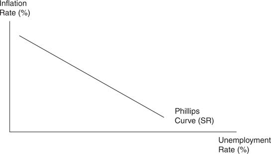
Figure 9.20
Supply Shocks and the Phillips Curve
We saw that when SRAS shifts to the right, holding AD constant, both the price level and unemployment rate fall. On the other hand, when SRAS shifts to the left, we get stagflation because inflation and unemployment rates are both rising. Figure 9.21 shows how supply shocks shift the Phillips curve inward when SRAS shifts to the right, and outward when SRAS shifts to the left.
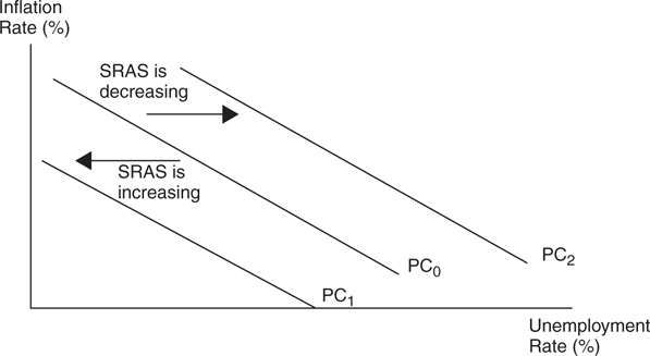
Figure 9.21
The Long-Run Phillips Curve
The AD and AS model presumes that the long-run AS curve is vertical and located at full employment. As a result, the Phillips curve in the long run is also vertical at the natural rate of employment. You might recall that the natural rate of employment is the unemployment rate where cyclical unemployment is zero. Suppose this occurs at a measured unemployment rate of 4 percent. Figure 9.22 illustrates the long-run Phillips curve.
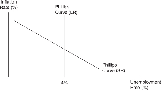
Figure 9.22
Expectations
The idea that there is, in the short term, an inverse relationship between inflation and unemployment, and in the long term, unemployment is always at the natural rate can be confusing. The reason is that sometimes a gap exists between the actual rate of inflation and the expected rate of inflation. Inflationary expectations play a role here in the derivation of the long-run Phillips curve. Figure 9.23 illustrates this concept with an example.
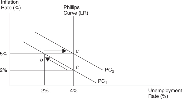
Figure 9.23
The expected inflation rate is 2 percent at a 4 percent natural rate of unemployment (point a ). If AD unexpectedly rises, this drives up the rate of inflation to 5 percent, and as a result, firms are earning higher profits. Firms respond with more hiring, and this temporarily drops the unemployment rate to 2 percent (point b ). This is seen as a movement along the short-run PC above from a to b .
The point at 5 percent inflation and 2 percent unemployment will not last. Workers realize that their real wages are falling and insist on a raise! As wages rise, the profits of firms begin to fall, and so too does employment back to the natural rate of 4 percent (point c ). At this point both actual and expected inflation is 5 percent. Another short-run Phillips curve runs through this point. Points a and c must lie on one long-run Phillips curve, and that curve must be vertical. The process can repeat itself if AD continues to increase, or it can reverse itself if AD falls. You might notice that this adjustment from a point on the SRPC back to the LRPC follows the adjustment from a short-run equilibrium to the long-run equilibrium in the AD/AS model.
What happens if citizens and firms expect a higher rate of inflation than the actual rate? Expecting higher prices in the future, consumers and firms increase purchasing now and AD increases, which serves to increase the price level. The expectation in this case is really a self-fulfilling prophecy.
![]() Review Questions
Review Questions
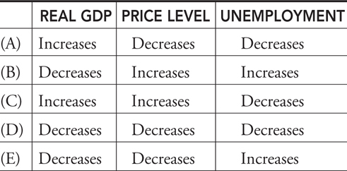
1 . Using the model of AD and AS, what happens in the short run to real GDP, the price level, and unemployment with more consumption spending (C )?
2 . Which is the best way to describe the AS curve in the long run?
(A) Always vertical in the long run.
(B) Always upward sloping because it follows the Law of Supply.
(C) Always horizontal.
(D) Always downward sloping.
(E) Without more information we cannot predict how it looks in the long run.
3 . Stagflation most likely results from
(A) increasing AD with constant SRAS.
(B) decreasing SRAS with constant AD.
(C) decreasing AD with constant SRAS.
(D) a decrease in both AD and SRAS.
(E) an increase in both AD and SRAS.
4 . Equilibrium real GDP is far below full employment, and the government lowers household taxes. Which is the likely result?
(A) Unemployment falls with little inflation.
(B) Unemployment rises with little inflation.
(C) Unemployment falls with rampant inflation.
(D) Unemployment rises with rampant inflation.
(E) No change occurs in unemployment or inflation.
5 . What is the main contrast between the short-run and long-run Phillips curve?
(A) In the short run there is a positive relationship between inflation and unemployment, and in the long run the relationship is negative.
(B) In the short run there is a positive relationship between inflation and unemployment, and in the long run the relationship is constant.
(C) In the short run there is a negative relationship between inflation and unemployment, and in the long run the relationship is positive.
(D) In the short run there is a negative relationship between inflation and unemployment, and in the long run the relationship is constant.
(E) In the short run there is a constant relationship between inflation and unemployment, and in the long run the relationship is negative.
6 . The effect of the spending multiplier is lessened if
(A) the price level is constant with an increase in aggregate demand.
(B) the price level falls with an increase in aggregate supply.
(C) the price level is constant with an increase in long-run aggregate supply.
(D) the price level falls with an increase in both aggregate demand and aggregate supply.
(E) the price level rises with an increase in aggregate demand.
![]() Answers and Explanations
Answers and Explanations
1 . C —An increase in consumption spending increases the AD curve, or shifts it to the right. Along the SRAS curve, we see increasing real GDP, a rising aggregate price level, and a lower unemployment rate.
2 . A —All resources are employed at full employment in the long run, so firms cannot respond to an increase in the price level by increasing production. Thus, any increase in prices cannot increase production in the long run, and so AS is assumed to be vertical. Any short-run discrepancy in GDP, above or below, full employment adjusts back to GDPf in the long run.
3 . B —Stagflation is an increase in the price level and an increase in unemployment. This is most often the result of falling SRAS and a constant AD. Choice D is incorrect because a simultaneous decrease in AD puts downward pressure on the price level, which offsets the upward pressure from falling SRAS.
4 . A —A deep recession describes macroeconomic equilibrium in the horizontal section of SRAS. Here, rising AD increases real GDP, and lowers unemployment, with little inflation.
5 . D —The short-run Phillips curve is downward sloping but the long-run Phillips curve is vertical.
6 . E —The full spending multiplier effect of an increase in AD is felt only if there is no rise in the price.
![]() Rapid Review
Rapid Review
Aggregate demand (AD): The inverse relationship between all spending on domestic output and the average price level of that output. AD measures the sum of consumption spending by households, investment spending by firms, government purchases of goods and services, and net exports (exports minus imports).
Foreign sector substitution effect: When the average price of U.S. output increases, consumers naturally begin to look for similar items produced elsewhere.
Interest rate effect: If the average price level rises, consumers and firms might need to borrow more money for spending and capital investment, which increases the interest rate and delays current consumption. This postponement reduces current consumption of domestic production as the price level rises.
Wealth effect: As the average price level rises, the purchasing power of wealth and savings begins to fall. Higher prices therefore tend to reduce the quantity of domestic output purchased.
Determinants of AD: AD is a function of the four components of domestic spending: C, I, G , and (X – M ). If any of these components increases (decreases), holding the others constant, AD increases (decreases), or shifts to the right (left).
Short-run aggregate supply (SRAS): The positive relationship between the level of domestic output produced and the average price level of that output.
Macroeconomic short run: A period of time during which the prices of goods and services are changing in their respective markets, but the input prices have not yet adjusted to those changes in the product markets. In the short run, the SRAS curve is typically drawn as upward sloping.
Macroeconomic long run: A period of time long enough for input prices to have fully adjusted to market forces. In this period, all product and input markets are in a state of equilibrium and the economy is operating at full employment (GDPf ). Once all markets in the economy have adjusted and there exists this long-run equilibrium, the LRAS curve is vertical at GDPf .
Determinants of AS: AS is a function of many factors that impact the production capacity of the nation. If these factors make it easier, or less costly, for a nation to produce, AS shifts to the right. If these factors make it more difficult, or more costly, for a nation to produce, AS shifts to the left.
Macroeconomic equilibrium: Occurs when the quantity of real output demanded is equal to the quantity of real output supplied. Graphically this is at the intersection of AD and SRAS. Equilibrium can exist at, above, or below full employment.
Recessionary gap: The amount by which full-employment GDP exceeds equilibrium GDP.
Inflationary gap: The amount by which equilibrium GDP exceeds full-employment GDP.
Demand-pull inflation: This inflation is the result of stronger consumption from all sectors of AD as it continues to increase in the upward-sloping range of SRAS. The price level begins to rise, and inflation is felt in the economy.
Deflation: A sustained falling price level, usually due to severely weakened aggregate demand and a constant SRAS.
Recession: In the AD and AS model, a recession is typically described as falling AD with a constant SRAS curve. Real GDP falls far below full employment levels and the unemployment rate rises.
Supply-side boom: When the SRAS curve shifts outward and the AD curve stays constant, the price level falls, real GDP increases and the unemployment rate falls.
Stagflation: A situation in the macroeconomy when inflation and the unemployment rate are both increasing. This is most likely the cause of falling SRAS while AD stays constant.
Supply shocks: A supply shock is an economy-wide phenomenon that affects the costs of firms and the position of the SRAS curve, either positively or negatively.
Phillips curve: A graphical device that shows the relationship between inflation and the unemployment rate. In the short run it is downward sloping, and in the long run it is vertical at the natural rate of unemployment.