Advanced Calculus of Several Variables (1973)

Part II. Multivariable Differential Calculus

Our study in Chapter I of the geometry and topology of provides an adequate foundation for the study in this chapter of the differential calculus of mappings from one Euclidean space to another. We will find that the basic idea of multivariable differential calculus is the approximation of nonlinear mappings by linear ones.

This idea is implicit in the familiar single-variable differential calculus. If the function is differentiable at a, then the tangent line at (a, f(a)) to the graph y = f(x) in is the straight line whose equation is

The right-hand side of this equation is a linear function of x − a; we may regard

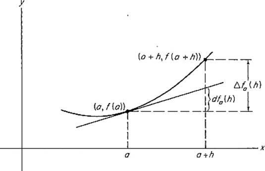
Figure 2.1

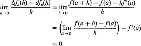
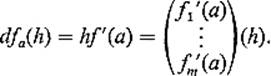
it as a linear approximation to the actual change f(x) − f(a) in the value of f between a and x. To make this more precise, let us write h = x − a, Δf_a(h) = f(a + h) − f(a), and df_a(h) = f′(a)h (see Fig. 2.1). The linear mapping , defined by df_a(h) = f′(a)h, is called the differential of f at a; it is simply that linear mapping whose matrix is the derivative f′(a) of f at a (the matrix of a linear mapping being just a real number). With this terminology, we find that when h is small, the linear change df_a(h) is a good approximation to the actual change Δf_a(h), in the sense that

Roughly speaking, our point of view in this chapter will be that a mapping is (by definition) differentiable at a if and only if it has near a an appropriate linear approximation . In this case df_a will be called the differential of f at a; its (m × n) matrix will be called the derivative of f at a, thus preserving the above relationship between the differential (a linear mapping) and the derivative (its matrix). We will see that this approach is geometrically well motivated, and permits the basic ingredients of differential calculus (for example, the chain rule, etc.) to be developed and utilized in a multivariable setting.

Chapter 1. CURVES IN R

We consider first the special case of a mapping . Motivated by curves in and , one may think of a curve in , traced out by a moving point whose position at time t is the point , and attempt to define its velocity at time t. Just as in the single-variable case, m = 1, this problem leads to the definition of the derivative f′ of f. The change in position of the particle from time a to time a + h is described by the vector f(a + h) − f(a), so the average velocity of the particle during this time interval is the familiar-looking difference quotient

whose limit (if it exists) as h → 0 should (by definition) be the instantaneous velocity at time a. So we define

if this limit exists, in which case we say that f is differentiable at . The derivative vector f′(a) of f at a may be visualized as a tangent vector to the image curve of f at the point f(a) (see Fig. 2.2); its length f′(a) is the speed at time t = a of the moving point f(t), so f′(a) is often called the velocity vector at time a.

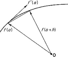
Figure 2.2

If the derivative mapping is itself differentiable at a, its derivative at a is the second derivative f″ (a) of f at a. Still thinking of f in terms of the motion of a moving point (or particle) in , f″(a) is often called the acceleration vector at time a. Exercises 1.3 and 1.4 illustrate the usefulness of the concepts of velocity and acceleration for points moving in higher-dimensional Euclidean spaces.

By Theorem 7.1 of Chapter I (limits in may be taken coordinatewise), we see that is differentiable at a if and only if each of its coordinate functions f₁, . . . , f_m is differentiable at a, in which case

That is, the differentiable function may be differentiated coordinate-wise. Applying coordinatewise the familiar facts about derivatives of real-valued functions, we therefore obtain the results listed in the following theorem.

Theorem 1.1 Let f and g be mappings from to , and , all differentiable. Then

and

Formula (5) is the chain rule for the composition .

Notice the familiar pattern for the differentiation of a product in formulas (3) and (4). The proofs of these formulas are all the same—simply apply componentwise the corresponding formula for real-valued functions. For example, to prove (5), we write

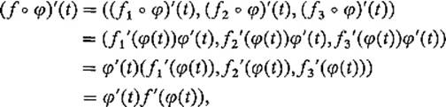
applying componentwise the single-variable chain rule, which asserts that

if the functions f, are differentiable at g(t) and t respectively.

We see below (Exercise 1.12) that the mean value theorem does not hold for vector-valued functions. However it is true that two vector-valued functions differ only by a constant (vector) if they have the same derivative; we see this by componentwise application of this fact for real-valued functions.

The tangent line at f(a) to the image curve of the differentiable mapping is, by definition, that straight line which passes through f(a) and is parallel to the tangent vector f′(a). We now inquire as to how well this tangent line approximates the curve close to f(a). That is, how closely does the mapping h → f(a) + hf′(a) of into (whose image is the tangent line) approximate the mapping h → f(a + h)? Let us write

for the actual change in f from a to a + h, and

for the linear (as a function of h) change along the tangent line. Then Fig. 2.3 makes it clear that we are simply asking how small the difference vector

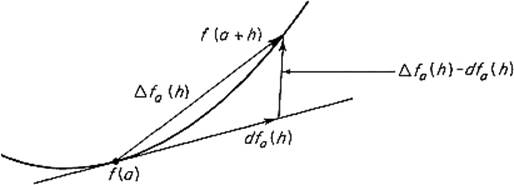
Figure 2.3

Δf_a(h) − df_a(h) is when h is small. The answer is that it goes to zero even faster than h does. That is,

by the definition of f′(a). Noting that is a linear mapping, we have proved the “only if” part of the following theorem.

Theorem 1.2 The mapping is differentiable at if and only if there exists a linear mapping such that

in which case L is defined by L(h) = df_a(h) = hf′(a).

To prove the “if” part, suppose that there exists a linear mapping satisfying (6). Then there exists such that L is defined by L(h) = hb; we must show that f′(a) exists and equals b. But

by (6).

If is differentiable at a, then the linear mapping , defined by df_a(h) = hf′(a), is called the differential of f at a. Notice that the derivative vector f′(a) is, as a column vector, the matrix of the linear mapping df_a, since

When in the next section we define derivatives and differentials of mappings from to , this relationship between the two will be preserved—the differential will be a linear mapping whose matrix is the derivative.

The following discussion provides some motivation for the notation df_a for the differential of f at a. Let us consider the identity function → , and write x for its name as well as its value at x. Since its derivative is 1 everywhere, its differential at a is defined by

If f is real-valued, and we substitute h = dx_a(h) into the definition of , we obtain

so the two linear mappings df_a and f′(a) dx_a are equal,

If we now use the Leibniz notation f′(a) = df/dx and drop the subscript a, we obtain the famous formula

which now not only makes sense, but is true! It is an actual equality of linear mappings of the real line into itself.

Now let f and g be two differentiable functions from to , and write h = g f for the composition. Then the chain rule gives

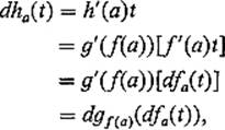
so we see that the single-variable chain rule takes the form

In brief, the differential of the composition h = g f is the composition of the differentials of g and f. It is this elegant formulation of the chain rule that we will generalize in Section 3 to the multivariable case.

Exercises

1.1Let f : be a differentiable mapping with f′(t) ≠ 0 for all . Let p be a fixed point not on the image curve of f as in Fig. 2.4. If q = f(t₀) is the point of the curve closest to p, that is, if for all , show that the vector p − q is orthogonal to the curve at q. Hint: Differentiate the function .

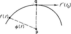
Figure 2.4

1.2(a)Let and be two differentiable curves, with f′(t) ≠ 0 and g′(t) ≠ 0 for all . Suppose the two points p = f(s₀) and q = g(t₀) are closer than any other pair of points on the two curves. Then prove that the vector p − q is orthogonal to both velocity vectors f′(s₀) and g′(t₀). Hint: The point (s₀, t₀) must be a critical point for the function defined by .
(b)Apply the result of (a) to find the closest pair of points on the “skew” straight lines in defined by f(s) = (s, 2s, −s) and g(t) = (t + 1, t − 2, 2t + 3).

1.3Let be a conservative force field on , meaning that there exists a continuously differentiable potential function such that F(x) = −V(x) for all [recall that V = (∂V/∂x₁, . . . , ∂V/∂x_n)]. Call the curve a “quasi-Newtonian particle” if and only if there exist constants m₁, m₂, . . . , m_n, called its “mass components,” such that

for each i = 1, . . . , n. Thus, with respect to the x_i-direction, it behaves as though it has mass m_i. Define its kinetic energy K(t) and potential energy P(t) at time t by

Now prove that the law of the conservation of energy holds for quasi-Newtonian particles, that is, K + P = constant. Hint: Differentiate K(t) + P(t), using the chain rule in the form P′(t) = V((t)) · ′(t), which will be verified in Section 3.

1.4(n-body problem) Deduce from Exercise 1.3 the law of the conservation of energy for a system of n particles moving in (without colliding) under the influence of their mutual gravitational attractions. You may take n = 2 for brevity, although the method is general. Hint: Denote by m₁and m₂ the masses of the two particles, and by r₁ = (x₁, x₂, x₃) and r₂ = (x₄, x₅, x₆) their positions at time t. Let r₁₂ = r₁ − r₂ be the distance between them. We then have a quasi-Newtonian particle in with mass components m₁, m₁, m₁, m₂, m₂, m₂ and force field F defined by

for . If

verify that F = −V. Then apply Exercise 1.3 to conclude that

Remark: In the general case of a system of n particles, the potential function would be

where r_ij = r_j − r_j.

1.5If is linear, prove that f′(a) exists for all , with df_a = f.

1.6If L₁ and L₂ are two linear mappings from ro ⁿ satisfying formula (6), prove that L₁ = L₂. Hint: Show first that

1.7Let f, both be differentiable at a.

(a)Show that d(fg)_a = g(a) df_a + f(a) dg_a.

(b)Show that

1.8Let γ(t) be the position vector of a particle moving with constant acceleration vector γ″(t) = a. Then show that , where p₀ = γ(0) and v₀ = γ′(0). If a = 0, conclude that the particle moves along a straight line through p₀ with velocity vector v₀ (the law of inertia).

1.9Let γ: → ⁿ be a differentiable curve. Show that γ(t) is constant if and only if γ(t) and γ′(t) are orthogonal for all t.

1.10Suppose that a particle moves around a circle in the plane ², of radius r centered at 0, with constant speed v. Deduce from the previous exercise that γ(t) and γ″(t) are both orthogonal to γ″(t), so it follows that γ″(t) = k(t)γ(t). Substitute this result into the equation obtained by differentiating γ(t) · γ′(t) = 0 to obtain k = −v²/r². Thus the acceleration vector always points towards the origin and has constant length v²/r.

1.11Given a particle in ³ with mass m and position vector γ(t), its angular momentum vector is L(t) = γ(t) × mγ′(t), and its torque is T(t) = γ(t) × mγ″(t).

(a)Show that L′(t) = T(t), so the angular momentum is constant if the torque is zero (this is the law of the conservation of angular momentum).

(b)If the particle is moving in a central force field, that is, γ(t) and γ″(t) are always collinear, conclude from (a) that it remains in some fixed plane through the origin.

1.12Consider a particle which moves on a circular helix in ³ with position vector

(a)Show that the speed of the particle is constant.

(b)Show that its velocity vector makes a constant nonzero angle with the z-axis.

(c)If t₁ = 0 and t₂ = 2π/Π, notice that γ(t₁) = (a, 0, 0) and γ(t₂) = (a, 0, 2πb), so the vector γ(t₂) − γ(t₁) is vertical. Conclude that the equation

cannot hold for any . Thus the mean value theorem does not hold for vector-valued functions.