Advanced Calculus of Several Variables (1973)

Part II. Multivariable Differential Calculus

Chapter 4. LAGRANGE MULTIPLIERS AND THE CLASSIFICATION OF CRITICAL POINTS FOR FUNCTIONS OF TWO VARIABLES

We saw in Section 2 that a necessary condition, that the differentiable function f : have a local extremum at the point p, is that p be a critical point for f, that is, that f(p) = 0. In this section we investigate sufficientconditions for local maxima and minima of functions of two variables. The general case (functions of n variables) will be treated in Section 8.

It turns out that we must first consider the special problem of maximizing or minimizing a function of the form

called a quadratic form, at the points of the unit circle x² + y² = 1. This is a special case of the general problem of maximizing or minimizing one function on the “zero set” of another function. By the zero set g(x, y) = 0 of the function g : is naturally meant the set . The important fact about a zero set is that, under appropriate conditions, it looks, at least locally, like the image of a curve.

Theorem 4.1 Let S be the zero set of the continuously differentiable function g : , and suppose p is a point of S where g(p) ≠ 0. Then there is a rectangle Q centered at p, and a differentiable curve φ : with φ(0) = pand φ′(0) ≠ 0, such that S and the image of φ agree inside Q. That is, a point of Q lies on the zero set S of g if and only if it lies on the image of the curve φ (Fig. 2.16).

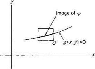
Figure 2.16

Theorem 4.1 is a consequence of the implicit function theorem which will be proved in Chapter III. This basic theorem asserts that, if g : is a continuously differentiable function and p a point where g(p) = 0 and D₂ g(p) ≠ 0, then in some neighborhood of p the equation g(x, y) = 0 can be “solved for y as a continuously differentiable function of x.” That is, there exists a function y = h(x) such that, inside some rectangle Q centered at p, the zero set S of g agrees with the graph of h. Note that, in this case, the curve φ(t) = (t, h(t)) satisfies the conclusion of Theorem 4.1.

The roles of x and y in the implicit function theorem can be reversed. If D₁g(p) ≠ 0, the conclusion is that, in some neighborhood of p, the equation g(x, y) = 0 can be “solved for x as a function of y.” If x = k(y) is this solution, then φ(t) = (k(t), t) is the desired curve in Theorem 4.1.

Since the hypothesis g(p) ≠ 0 in Theorem 4.1 implies that either D₁g(p) ≠ 0 or D₂g(p) ≠ 0, we see that Theorem 4.1 does follow from the implicit function theorem.

For example, suppose that g(x, y) = x² + y² − 1, so the zero set S is the unit circle. Then, near (1, 0), S agrees with the graph of x = (1 − y²)^1/2, while near (0, −1) it agrees with the graph of y = − (1 − x²)^1/2 (see Fig. 2.17).

The condition g(p) ≠ 0 is necessary for the conclusion of Theorem 4.1. For example, if g(x, y) = x² + y², or if g(x, y) = x² − y², then 0 is a critical

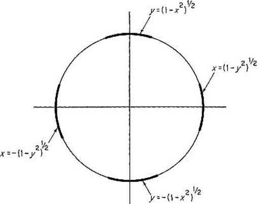
Figure 2.17

point in the zero set of g, and S does not look like the image of a curve near 0 (see Fig. 2.18).

We are now ready to study the extreme values attained by the function f on the zero set S of the function g. We say that f attains its maximum value (respectively, minimum value) on S at the point (respectively, ).

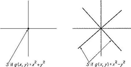
Figure 2.18

Theorem 4.2 Let f and g be continuously differentiable functions on ². Suppose that f attains its maximum or minimum value on the zero set S of g at the point p where g(p) ≠ 0. Then

for some number λ.

The number λ is called a “Lagrange multiplier.”

PROOF Let φ : be the differentiable curve given by Theorem 4.1. Then g(φ(t)) = 0 for t sufficiently small, so the chain rule gives

Since f attains a maximum or minimum on S at p, the function h(t) = f(φ(t)) attains a maximum or minimum at 0. Hence h′(0) = 0, so the chain rule gives

Thus the vectors f(p) and g(p) ≠ 0 are both orthogonal to the nonzero vector φ′(0), and are therefore collinear. This implies that (1) holds for some .

(Theorem 4.2 provides a recipe for locating the points p = (x, y) at which f attains its maximum and minimum values (if any) on the zero set of g (provided they are attained at points where the gradient vector g ≠ 0). The vector equation (1) gives two scalar equations in the unknowns x, y, λ, while g(x, y) = 0 is a third equation. In principle these three equations can be solved for x, y, λ. Each solution (x, y, λ) gives a candidate (x, y) for an extreme point. We can finally compare the values of f at these candidate points to ascertain where its maximum and minimum values on S are attained.

Example 1 Suppose we want to find the point(s) of the rectangular hyperbola xy = 1 which are closest to the origin. Take f(x, y) = x² + y² (the square of the distance from 0) and g(x, y) = xy − 1. Then f = (2x, 2y) and g = (y, x), so our three equations are

From the third equation, we see that x ≠ 0 and y ≠ 0, so we obtain

from the first two equations. Hence x² = y². Since xy = 1, we obtain the two solutions (1, 1) and (−1, −1).

Example 2 Suppose we want to find the maximum and minimum values of f(x, y) = xy on the circle g(x, y) = x² + y² − 1 = 0. Then f = (y, x) and g = (2x, 2y), so our three equations are

From the first two we see that if either x or y is zero, then so is the other. But the third equation implies that not both are zero, so it follows that neither is. We therefore obtain

from the first two equations. Hence (since x² + y² = 1). This gives four solutions: . Evaluating f at these four points, we find that f attains its maximum value of at the first and third of these points, and its minimum value of at the other two (Fig. 2.19).

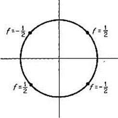
Figure 2.19

Example 3 The general quadratic form f(x, y) = ax² + 2bxy + cy² attains both a maximum value and a minimum value on the unit circle g(x, y) = x² + y² − 1 = 0, because f is continuous and the circle is closed and bounded (see Section I.8). Applying Theorem 4.2, we obtain the three equations

The first two of these can be written in the form

Thus the two vectors (a − λ, b) and (b, c − λ) are both orthogonal to the vector (x, y), which is nonzero because x² + y² = 1. Hence they are collinear, and it follows easily that

This is a quadratic equation whose two roots are

It is easily verified that

If ac − b² < 0, then λ₁ and λ₂ have different signs. If ac − b² > 0, then they have the same sign, the sign of a and c, which have the same sign because .

Now, instead of proceeding to solve for x and y, let us just consider a solution (x_i, y_i, λ_i) of (2). Then

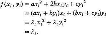
Thus λ₁ and λ₂ are the maximum and minimum values of f(x, y) on x² + y² = 1, so we do not need to solve for x and y explicitly after all.

To summarize Example 3, we see that the maximum and minimum values of (x, y) = ax² + 2bxy + cy² on the unit circle

(i) are both positive if a > 0 and ac − b² > 0,

(ii) are both negative if a < 0 and ac − b² > 0,

(iii) have different signs if ac − b² < 0.

A quadratic form is called positive-definite if f(x, y) > 0 unless x = y = 0, negative-definite if f(x, y) < 0 unless x = y = 0, and nondefinite if it has both positive and negative values. If (x, y) is a point not necessarily on the unit circle, then

Consequently we see that the character of a quadratic form is determined by the signs of the maximum and minimum values which it attains on the unit circle. Combining this remark with (i), (ii), (iii) above, we have proved the following theorem.

Theorem 4.3 The quadratic form f(x, y) = ax² + 2bxy + cy² is

(i) positive definite if a > 0 and ac − b² > 0,

(ii) negative-definite if a < 0 and ac − b² > 0,

(iii) nondefinite if ac − b² < 0.

Now we want to use Theorem 4.3 to derive a “second-derivative test” for functions of two variables. In addition to Theorem 4.3, we will need a certain type of Taylor expansion for twice continuously differentiable functions of two variables. The function f : is said to be twice continuously differentiable at p if it has continuous partial derivatives in a neighborhood of p, which are themselves continuously differentiable at p. The partial derivatives of D₁ f are D₁(D₁ f) = D₁²f and D₂ D₁ f, and the partial derivatives of D₂ f are D₁ D₂ f and D₂ D₂ f = D₂²f.

Now suppose that f is twice continuously differentiable on some disk centered at the point p = (a, b), and let q = (a + h, b + k) be a point of this disk. Define where c(t) = (a + th, b + tk) (see Fig. 2.20).

Taylor's formula for single-variable functions will be reviewed in Section 6. Applied to φ on the interval [0, 1], it gives

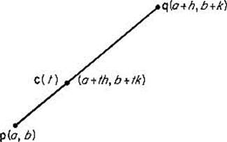
Figure 2.20

for some . An application of the chain rule first gives

and then

Since c(0) = (a, b) and c(τ) = (a + τh, b + τk), (4) now becomes

where

This is the desired Taylor expansion of f. We could proceed in this manner to derive the general kth degree Taylor formula for a function of two variables, but will instead defer this until (Section 7 since (5) is all that is needed here.

We are finally ready to state the “second-derivative test” for functions of two variables. Its proof will involve an application of Theorem 4.3 to the quadratic form

Let us write

and call Δ the determinant of the quadratic form q.

Theorem 4.4 Let f : be twice continuously differentiable in a neighborhood of the critical point p = (a, b). Then f has

(i)a local minimum at p if Δ > 0 and D₁²f(p) > 0,

(ii)a local maximum at p if Δ > 0 and D₁²f(p) < 0,

(iii)neither a local minimum nor a local maximum at p if Δ < 0 (so in this case p is a “saddle point” for f).

If Δ = 0, then the theorem does not apply.

PROOF Since the functions D₁²f(x, y) and

are continuous and nonzero at p, we can choose a circular disk centered at p and so small that each has the same sign at every point of this disk. If (a + h, b + k) is a point of this disk, then (5) gives

because D₁f(a, b) = D₂f(a, b) = 0.

In case (i), both D₁²f(a + τh, b + τk) and the determinant Δ(a + τh, b + τk) of q_τ are positive, so Theorem 4.3(i) implies that the quadratic form q_τ is positive-definite. We therefore see from (7) that f(a + h, b + k) > f(a, b). This being true for all sufficiently small h and k, we conclude that f has a local minimum at p.

The proof in case (ii) is the same, except that we apply Theorem 4.3(ii) to show that q_τ is negative-definite, so f(a + h, b + k) < f(a, b) for all h and k sufficiently small.

In case (iii), Δ(a + τh, b + τk) < 0, so q_τ is nondefinite by Theorem 4.3(iii). Therefore q_τ(h, k) assumes both positive and negative values for arbitrarily small values of h and k, so it is clear from (7) that f has neither a local minimum nor a local maximum at p.

Example 4 Let f(x, y) = xy + 2x − y. Then

so (1, −2) is the only critical point. Since D₁²f = D₂²f = 0 and D₁D₂f = 1, Δ < 0, so f has neither a local minimum nor a local maximum at (1, −2).

The character of a given critical point can often be ascertained without application of Theorem 4.4. Consider, for example, a function f which is defined on a set D in the plane that consists of all points on and inside some simple closed curve C (that is, C is a closed curve with no self-intersections). We proved in Section I.8 that, if f is continuous on such a set D, then it attains both a maximum value and a minimum value at points of D (why?).

Now suppose in addition that f is zero at each point of C, and positive at each point inside C. Its maximum value must then be attained at an interior point which must be a critical point. If it happens that f has only a single critical point p inside C, then f must attain its (local and absolute) maximum value at at p, so we need not apply Theorem 4.4.

Example 5 Suppose that we want to prove that the cube of edge 10 is the rectangular solid of value 1000 which has the least total surface area A. If x, y, z are the dimensions of the box, then xyz = 1000 and A = 2xy + 2xz + 2yz. Hence the function

defined on the open first quadrant x > 0, y > 0, gives the total surface area of the rectangular solid with volume 1000 whose base has dimensions x and y.

It is clear that we need not consider either very small or very large values of x and y. For instance while the cube of edge 10 has total surface area 600. So we consider f on the set D pictured in Fig. 2.21. Since at each point of the boundary C of D,

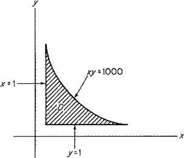
Figure 2.21

and since f attains values less than 2000 inside C [f(10, 10) = 600], it follows that f must attain its minimum value at a critical point interior to D. Now

We find easily that the only critical point is (10, 10), so f(10, 10) = 600 (the total surface area of the cube of edge 10) must be the minimum value of f.

In general, if f is a differentiable function on a region D bounded by a simple closed curve C, then f may attain its maximum and minimum values on D either at interior points of D or at points of the boundary curve C. The procedure for maximizing or minimizing f on D is therefore to locate both the critical points of f that are interior to C, and the possible maximum–minimum points on C (by the Lagrange multiplier method), and finally to compare the values of f at all of the candidate points so obtained.

Example 6 Suppose we want to find the maximum and minimum values of f(x, y) = xy on the unit disk . In Example 2 we have seen that the maximum and minimum values of f(x, y) on the boundary x²+ y² = 1 of D are and , respectively. The only interior critical point is the origin where f(0, 0) = 0. Thus and are the extreme values of fon D.

Exercises

4.1Find the shortest distance from the point (1, 0) to a point of the parabola y² = 4x.

4.2Find the points of the ellipse x²/9 + y²/4 = 1 which are closest to and farthest from the point (1, 0).

4.3Find the maximal area of a rectangle (with vertical and horizontal sides) inscribed in the ellipse x²/a² + y²/b² = 1.

4.4The equation 73x² + 72xy + 52y² = 100 defines an ellipse which is centered at the origin, but has been rotated about it. Find the semiaxes of this ellipse by maximizing and minimizing f(x, y) = x² + y² on it.

4.5(a) Show that if (x, y) is a point of the line segment .

(b) If a and b are positive numbers, show that . Hint: Apply (a) with x = a/(a + b), y = b/(a + b).

4.6(a) Show that log if (x, y) is a point of the unit circle x² + y² = 1 in the open first quadrant x > 0, y > 0. Hence for such a point.

(b) Apply (a) with x = a^1/2/(a + b)^1/2, y = b^1/2/(a + b)^1/2 to show again that if a > 0, b > 0.

4.7(a) Show that if x² + y² = 1 by finding the maximum and minimum values of f(x, y) = ax + by on the unit circle.

(b) Prove the Cauchy-Schwarz inequality

by applying (a) with x = c/(c² + d²)^1/2, y = d/(c² + d²)^1/2.

4.8Let C be the curve defined by g(x, y) = 0, and suppose g ≠ 0 at each point of C. Let p be a fixed point not on C, and let q be a point of C that is closer to p than any other point of C. Prove that the line through p and q is orthogonal to the curve C at q.

4.9Prove that, among all closed rectangular boxes with total surface area 600, the cube with edge 10 is the one with the largest volume.

4.10Show that the rectangular solid of largest volume that can be inscribed in the unit sphere is a cube.

4.11Find the maximum volume of a rectangular box without top, which has the combined area of its sides and bottom equal to 100.

4.12Find the maximum of the product of the sines of the three angles of a triangle, and show that the desired triangle is equilateral.

4.13If a triangle has sides of lengths x, y, z, so its perimeter is 2s = x + y + z, then its area A is given by A² = s(s − x)(s − y)(s − z). Show that, among all triangles with a given perimeter, the one with the largest area is equilateral.

4.14Find the maximum and minimum values of the function f(x, y) = x² − y² on the elliptical disk .

4.15Find and classify the critical points of the function .

4.16If x, y, z are any three positive numbers whose sum is a fixed number s, show that xyz (s/3)³by maximizing f(x, y) = xy(s − x − y) on the appropriate set. Conclude from this that , another case of the “arithmetic-geometric means inequality.”

4.17A wire of length 100 is cut into three pieces of lengths x, y, and 100 − x − y. The first piece is bent into the shape of an equilateral triangle, the second is bent into the shape of a rectangle whose base is twice its height, and the third is made into a square. Find the minimum of the sum of the areas if x > 0, y > 0, 100 − x − y > 0 (use Theorem 4.4 to check that you have a minimum). Find the maximum of the sum of the areas if we allow x = 0 or y = 0 or 100 − x − y = 0, or any two of these.

The remaining three exercises deal with the quadratic form

of Example 3 and Theorem 4.3.

4.18Let (x₁, y₁, λ₁) and (x₂, y₂, λ₂) be two solutions of the equations

which were obtained in Example 3. If λ₁ ≠ λ₂, show that the vectors v₁ = (x₁, y₁) and v₂ = (x₂, y₂) are orthogonal. Hint: Substitute (x₁, y₁, λ₁) into the first two equations of (2), multiply the two equations by x₂ and y₂ respectively, and then add. Now substitute (x₂, y₂, λ₂) into the two equations, multiply them by x₁ and y₁ and then add. Finally subtract the results to obtain (λ₁ − λ₂)v₁ · v₂ = 0.

4.19Define the linear mapping L : ² by

and note that f(x) = x · L(x) for all x. If v₁ and v₂ are as in the previous problem, show that

A vector, whose image under the linear mapping L : ² is a scalar multiple of itself, is called an eigenvector of L.

4.20Let v₁ and v₂ be the eigenvectors of the previous problem. Given x, let (u₁, u₂) be the coordinates of x with respect to axes through v₁ and v₂ (see Fig. 2.22). That is, u₁ and u₂ are the (unique) numbers such that

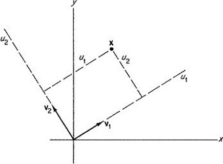
Figure 2.22

Substitute this equation into f(x) = x · L(x), and then apply the fact that v₁ and v₂ are eigenvectors of L to deduce that

Thus, in the new coordinate system, f is a sum or difference of squares.

4.21Deduce from the previous problem that the graph of equation ax² + 2bxy + cy² = 1 is

(a) an ellipse if ac − b² − > 0,

(b) a hyperbola if ac − b² < 0.