Advanced Calculus of Several Variables (1973)
Part V. Line and Surface Integrals; Differential Forms and Stokes' Theorem
Chapter 5. DIFFERENTIAL FORMS
We have seen that a differential 1-form ω on ![]() n is a mapping which associates with each point
n is a mapping which associates with each point ![]() a linear function ω(x) :
a linear function ω(x) : ![]() n →
n → ![]() , and that each linear function on
, and that each linear function on ![]() n is a linear combination of the differentials dx1, . . . , dxn, so
n is a linear combination of the differentials dx1, . . . , dxn, so
![]()
where a1, . . . , an are real-valued functions on ![]() n.
n.
A differential k-form α, defined on the set ![]() is a mapping which associates with each point
is a mapping which associates with each point ![]() an alternating k-multilinear function α(x) = αx on
an alternating k-multilinear function α(x) = αx on ![]() n. That is,
n. That is,
![]()
where λk(![]() n) denotes the set of all alternating k-multilinear functions on
n) denotes the set of all alternating k-multilinear functions on ![]() n. Since we have seen in Theorem 3.4 that every alternating k-multilinear function on
n. Since we have seen in Theorem 3.4 that every alternating k-multilinear function on ![]() n is a (unique) linear combination of the “multidifferentials” dxi, it follows that α(x) can be written in the form
n is a (unique) linear combination of the “multidifferentials” dxi, it follows that α(x) can be written in the form
![]()
where as usual [i] denotes summation over all increasing k-tuples i = (i1, . . . , ik) with ![]() , and each ai is a real-valued function on U. The differential k-form α is called continuous (or
, and each ai is a real-valued function on U. The differential k-form α is called continuous (or ![]() , etc.) provided that each of the coefficient functions ai is continuous (or
, etc.) provided that each of the coefficient functions ai is continuous (or ![]() , etc.).
, etc.).
For example, every differential 2-form α on ![]() 3 is of the form
3 is of the form
![]()
while every differential 3-form β on ![]() 3 is a scalar (function) multiple of the single multidifferential dx(1, 2, 3),
3 is a scalar (function) multiple of the single multidifferential dx(1, 2, 3),
![]()
Similarly, every differential 2-form on ![]() n is of the form
n is of the form
![]()
A standard and useful alternative notation for multidifferentials is
![]()
if i = (i1, . . . , ik); we think of the multidifferential dxi as a product of the differentials ![]() Recall that, if A is the n × k matrix whose column vectors are a1, . . . , ak, then
Recall that, if A is the n × k matrix whose column vectors are a1, . . . , ak, then
![]()
where Ai denotes the k × k matrix whose rth row is the irth row of A. If ir = is, then the rth and sth rows of Ai are equal, so
![]()
In terms of the product notation of (2) , it follows that
![]()
unless the integers i1, . . . , ik are distinct. In particular,
![]()
for each i = 1, . . . , n. Similarly,
![]()
since the sign of a determinant is changed when two of its rows are interchanged.
The multiplication of differentials extends in a natural way to a multiplication of differential forms. First we define
![]()
if i = (i1, . . . . , ik) and j = (j1, . . . , jl). Then, given a differential k-form
![]()
and a differential l-form
![]()
their product α ![]() β (sometimes called exterior product) is the differential (k + l)-form defined by
β (sometimes called exterior product) is the differential (k + l)-form defined by
![]()
This means simply that the differential forms α and β are multiplied together in a formal term-by-term way, using (5) and distributivity of multiplication over addition. Strictly speaking, the result of this process, the right-hand side of (6) , is not quite a differential form as defined in (1) , because the typical (k + l)-tuple (i, j) = (i1, . . . , ik, j1, . . . , jl) appearing in (6) is not necessarily increasing. However it is clear that, by use of rules (3) and (4) , we can rewrite the result in the form
![]()
with the summation being over all increasing (k + l)-tuples. Note that α ![]() β = 0 if k + l > n.
β = 0 if k + l > n.
It will be an instructive exercise for the student to deduce from this definition and the anticommutative property (4) that, if α is a k-form and β is an l-form, then
![]()
Example 1 Let α = a1 dx1 + a2 dx2 + a3 dx3 and β = b1 dx1 + b2 dx2 + b3 dx3 be two 1-forms on ![]() 3. Then
3. Then
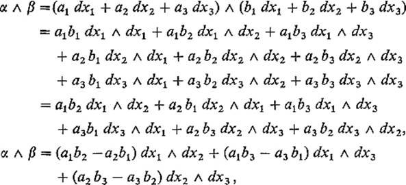
using (3) and (4) , respectively in the last two steps. Similarly, consider a 1-form ω = P dx + Q dy + R dz and 2-form α = A dx ![]() dy + B dx
dy + B dx ![]() dz + C dy
dz + C dy ![]() dz. Applying (3) to delete immediately each multidifferential that contains twice a single differential dx or dy or dz, we obtain
dz. Applying (3) to delete immediately each multidifferential that contains twice a single differential dx or dy or dz, we obtain
![]()
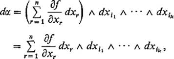
We next define an operation of differentiation for differential k-forms, extending our previous definitions in the case of 0-forms (or functions) on ![]() n and 1-forms on
n and 1-forms on ![]() 2. Recall that the differential of the
2. Recall that the differential of the ![]() function f:
function f: ![]() n →
n → ![]() is defined by
is defined by
![]()
Given a ![]() differential k-form
differential k-form ![]() defined on the open set
defined on the open set ![]() its differential dα is the (k + 1)-form defined on U by
its differential dα is the (k + 1)-form defined on U by
![]()
Note first that the differential operation is clearly additive,
![]()
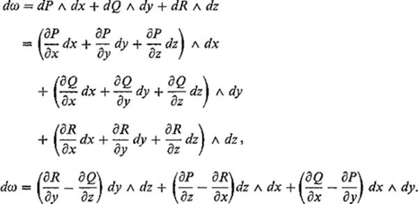
Example 2 If ω = P dx + Q dy + R dz, then
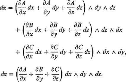
If α = A dy ![]() dz + B dz
dz + B dz ![]() dx + C dx
dx + C dx ![]() dy, then
dy, then
If ω is of class ![]() then, setting α = dω, we obtain
then, setting α = dω, we obtain
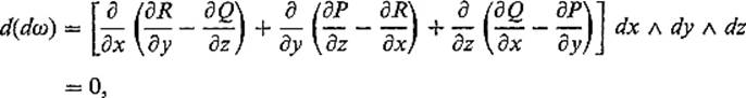
by the equality, under interchange of order of differentiation, of mixed second order partial derivatives of ![]() functions. The fact, that d(dω) = 0 if ω is a
functions. The fact, that d(dω) = 0 if ω is a ![]() differential 1-form in
differential 1-form in ![]() 3, is an instance of a quite general phenomenon.
3, is an instance of a quite general phenomenon.
Proposition 5.1 If α is a ![]() differential k-form on an open subset of
differential k-form on an open subset of ![]() n, then d(dα) = 0.
n, then d(dα) = 0.
PROOF Since d(β + γ) = dβ + dγ, it suffices to verify that d(dα) = 0 if
![]()
Then
so
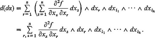
But since dxr ![]() dxs = −dxs
dxs = −dxs ![]() dxr, the terms in this latter sum cancel in pairs, just as in the special case considered in Example 2.
dxr, the terms in this latter sum cancel in pairs, just as in the special case considered in Example 2.
![]()
There is a Leibniz-type formula for the differential of a product, but with an interesting twist which results from the anticommutativity of the product operation for forms.
Proposition 5.2 If α is a differential k-form and β a differential l-form, both of class ![]() , then
, then
![]()
PROOF By the additivity of the differential operation, it suffices to consider the special case
![]()
where a and b are ![]() functions. Then
functions. Then
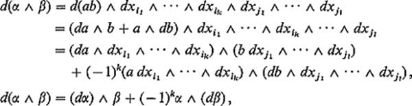
the (−1)k coming from the application of formula (7) to interchange the 1-form db and the k-form α in the second term.
![]()
Recall (from Section 1 ) that, if ω is a ![]() differential 1-form on
differential 1-form on ![]() n, and γ: [a, b] →
n, and γ: [a, b] → ![]() n is a
n is a ![]() path, then the integral of ω over γ is defined by
path, then the integral of ω over γ is defined by
![]()
We now generalize this definition as follows. If α is a ![]() differential k-form on
differential k-form on ![]() n, and φ: Q →
n, and φ: Q → ![]() n is a
n is a ![]() k-dimensional surface patch, then the integral of α over φ is defined by
k-dimensional surface patch, then the integral of α over φ is defined by
![]()
Note that, since the partial derivatives D1 φ, . . . , Dkφ are vectors in ![]() n, the right-hand side of (10) is the “ordinary” integral of a continuous real-valued function on the k-dimensional interval
n, the right-hand side of (10) is the “ordinary” integral of a continuous real-valued function on the k-dimensional interval ![]()
In the special case k = n, the following notational convention is useful. If α = f dx1 ![]() · · ·
· · · ![]() dxk is a
dxk is a ![]() differential k-form on
differential k-form on ![]() k, we write
k, we write
![]()
(“ordinary” integral on the right). In other words, ∫Q α is by definition equal to the integral of α over the identity (or inclusion) surface patch ![]() (see Exercise 5.7) .
(see Exercise 5.7) .
The definition in (10) is simply a concise formalization of the result of the following simple and natural procedure. To evaluate the integral
![]()
first make the substitutions ![]() throughout. After multiplying out and collecting coefficients, the final result is a differential k-form β = g du1
throughout. After multiplying out and collecting coefficients, the final result is a differential k-form β = g du1 ![]() · · ·
· · · ![]() duk on Q. Then
duk on Q. Then
![]()
Before proving this in general, let us consider the special case in which α = f dy ![]() dz is a 2-form on
dz is a 2-form on ![]() 3, and φ: Q →
3, and φ: Q → ![]() 3 is a 2-dimensional surface patch. Using uv-coordinates in
3 is a 2-dimensional surface patch. Using uv-coordinates in ![]() 2, we obtain
2, we obtain
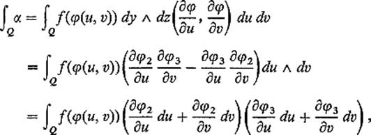
thus verifying (in this special case) the assertion of the preceding paragraph.
In order to formulate precisely (and then prove) the general assertion, we must define the notion of the pullback φ*(α) = φ*α, of the k-form α on ![]() n, under a
n, under a ![]() mapping
mapping ![]() This will be a generalization of the pullback defined in Section 2 for differential forms on
This will be a generalization of the pullback defined in Section 2 for differential forms on ![]() 2. We start by defining the pullback of a 0-form (or function) f or differential dxi by
2. We start by defining the pullback of a 0-form (or function) f or differential dxi by
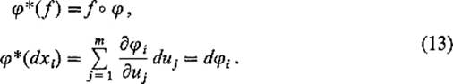
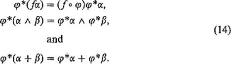
We can then extend the definition to arbitrary k-forms on ![]() n by requiring that
n by requiring that
Exercise 5.8 gives an important interpretation of this definition of the pullback operation.
Example 3 Let φ be a ![]() mapping from
mapping from ![]() to
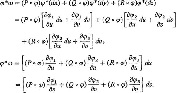
to ![]() If ω = P dx + Q dy + R dz, then
If ω = P dx + Q dy + R dz, then
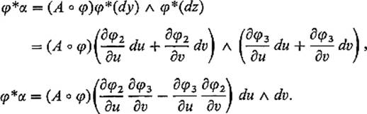
If α = A dy ![]() dz, then
dz, then
In terms of the pullback operation, what we want to prove is that
![]()
this being the more precise formulation of Eq. (12) . We will need the following lemma.
Lemma 5.3 Let ω1, . . . , ωk be k differential 1-forms on ![]() k, with
k, with
![]()
in u-coordinates. Then
![]()
where A is the k × k matrix (aij).
PROOF Upon multiplying out, we obtain
![]()
where the notation {j} signifies summation over all permutations j = (j1, . . . , jk) of (1, . . . , k). If σ(j) denotes the sign of the permutation j, then
![]()
so we have
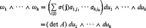
by the standard definition of det A.
![]()
Theorem 5.4 If φ : Q → ![]() n is a k-dimensional
n is a k-dimensional ![]() surface patch, and α is a differential k-form on
surface patch, and α is a differential k-form on ![]() n, then
n, then
![]()
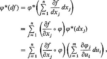
PROOF By the additive property of the pullback, it suffices to consider
![]()
Then
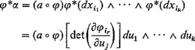
by Lemma 5.3 (here ![]() is the element in the rth row and jth column). Therefore, applying the definitions, we obtain
is the element in the rth row and jth column). Therefore, applying the definitions, we obtain
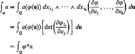
as desired.
![]()
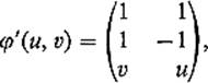
Example 4 Let ![]() and suppose φ : Q →
and suppose φ : Q → ![]() 3 is defined by the equations
3 is defined by the equations
![]()
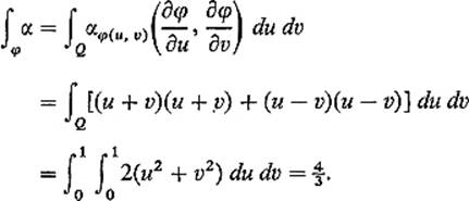
We compute the surface integral
![]()
in two different ways. First we apply the definition in Eq. (10) . Since
we see that
![]()
Therefore
Second, we apply Theorem 5.4 . The pullback φ*α is simply the result of substituting
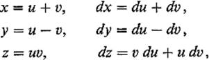
into α. So
![]()
Therefore Theorem 5.4 gives
![]()
Of course the final computation is the same in either case. The point is that Theorem 5.4 enables us to proceed by formal substitution, making use of the equations which define the mapping φ, instead of referring to the original definition of ∫φ α.
Theorem 5.4 is the k-dimensional generalization of Lemma 2.2(b) , which played an important role in the proof of Green‘s theorem in Section 2. Theorem 5.4 will play a similar role in the proof of Stokes’ theorem in Section 6 . We will also need the k-dimensional generalization of part (c) of Lemma 2.2 —the fact that the differential operation d commutes with pullbacks.
Theorem 5.5 If φ : ![]() m →
m → ![]() n is a
n is a ![]() mapping and α is a
mapping and α is a ![]() differential k-form on
differential k-form on ![]() n, then
n, then
![]()
PROOF The proof will be by induction on k. When k = 0, α = f, a ![]() function on
function on ![]() n, and φ*f = f
n, and φ*f = f ![]() φ, so
φ, so
![]()
But
which is the same thing.
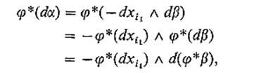
Supposing inductively that the result holds for (k − 1)-forms, consider the k-form
![]()
where ![]() . Then
. Then
![]()
by Proposition 5.2. Therefore
since φ*(dβ) = d(φ*β) by the inductive assumption. Since ![]() by (13) , we now have
by (13) , we now have
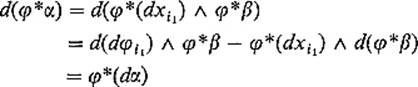
using Propositions 5.1 and 5.2.
![]()
Our treatment of differential forms in this section has thus far been rather abstract and algebraic. As an antidote to this absence of geometry, the remainder of the section is devoted to a discussion of the “surface area form” of an oriented smooth (![]() ) k-manifold in
) k-manifold in ![]() n. This will provide an example of an important differential form that appears in a natural geometric setting.
n. This will provide an example of an important differential form that appears in a natural geometric setting.
First we recall the basic definitions from Section 4 of Chapter III . A coordinate patch on the smooth k-manifold ![]() is a one-to-one
is a one-to-one ![]() mapping φ : U → M, where U is an open subset of
mapping φ : U → M, where U is an open subset of ![]() k, such that dφu has rank k for each
k, such that dφu has rank k for each ![]() this implies that [det(φ′(u)tφ′(u)]1/2 ≠ 0. An atlas for M is a collection {
this implies that [det(φ′(u)tφ′(u)]1/2 ≠ 0. An atlas for M is a collection {![]() i} of coordinate patches, the union of whose images covers M. An orientation for M is an atlas {
i} of coordinate patches, the union of whose images covers M. An orientation for M is an atlas {![]() i} such that the “change of coordinates” mapping, corresponding to any two of these coordinate patches
i} such that the “change of coordinates” mapping, corresponding to any two of these coordinate patches ![]() i and
i and ![]() j whose images
j whose images ![]() i(Ui) and
i(Ui) and ![]() j(Uj) overlap, has a positive Jacobian determinant. That is, if
j(Uj) overlap, has a positive Jacobian determinant. That is, if
![]()
then det T′ij > 0 wherever Tij is defined (see Fig. 5.29) . The pair (M, {![]() i}, is then called an oriented manifold. Finally, the coordinate patch φ : U → M is called orientation-preserving if it overlaps positively (in the above sense) with each of the
i}, is then called an oriented manifold. Finally, the coordinate patch φ : U → M is called orientation-preserving if it overlaps positively (in the above sense) with each of the ![]() i, and orientation-reversing if it overlaps negatively with each of the
i, and orientation-reversing if it overlaps negatively with each of the ![]() i (that is, the appropriate Jacobian determinants are negative at each point).
i (that is, the appropriate Jacobian determinants are negative at each point).
The surface area form of the oriented k-dimensional manifold ![]() is the differential k-form
is the differential k-form
![]()
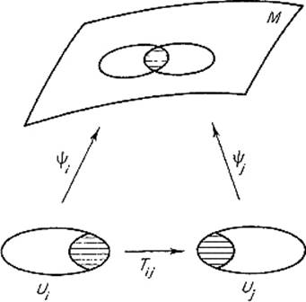
Figure 5.29
whose coefficient functions ni are defined on M as follows. Given i = (i1, . . . , ik) and ![]() choose an orientation-preserving coordinate patch φ : U → M such that
choose an orientation-preserving coordinate patch φ : U → M such that ![]() . Then
. Then
![]()
where
![]()
Example 5 Let M = S2, the unit sphere in ![]() 3. We use the spherical coordinates surface patch defined as usual by
3. We use the spherical coordinates surface patch defined as usual by
![]()
Here D = sin φ (see Example 3 in Section 4) . Hence
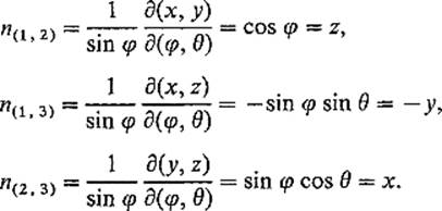
Thus the area form of S2 is
![]()
Of course we must prove that ni is well-defined. So let ![]() : V → M be a second orientation-preserving coordinate patch with
: V → M be a second orientation-preserving coordinate patch with ![]() If
If
![]()
then φ = ![]()
![]() T on
T on ![]() , so an application of the chain rule gives
, so an application of the chain rule gives
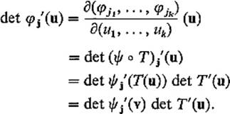
Therefore
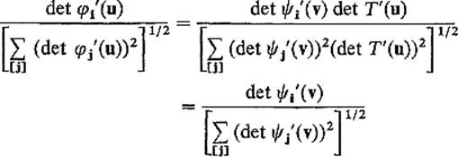
because det T′(u) > 0. Thus the two orientation-preserving coordinate patches φ and ![]() provide the same definition of ni(x).
provide the same definition of ni(x).
The following theorem tells why dA is called the “surface area form” of M.
Theorem 5.6 Let M be an oriented k-manifold in ![]() n with surface area form dA. If φ : Q → M is the restriction, to the k-dimensional interval
n with surface area form dA. If φ : Q → M is the restriction, to the k-dimensional interval ![]() , of an orientation-preserving coordinate patch, then
, of an orientation-preserving coordinate patch, then
![]()
PROOF The proof is simply a computation. Using the definition of dA, of the area a(φ), and of the integral of a differential form, we obtain
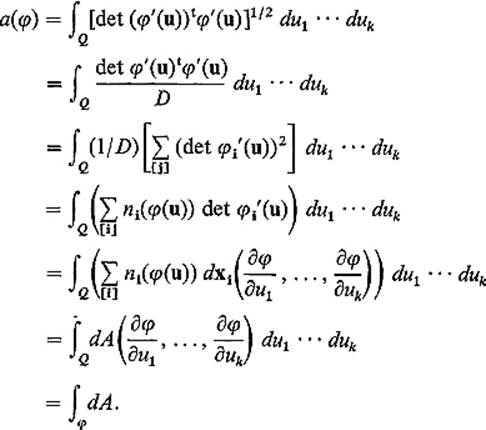
![]()
Recall that a paving of the compact smooth k-manifold M is a finite collection ![]() = {A1, . . . , Ar} of nonoverlapping k-cells such that
= {A1, . . . , Ar} of nonoverlapping k-cells such that ![]() . If M is oriented, then the paving
. If M is oriented, then the paving ![]() is called oriented provided that each of the k-cells Ai has a parametrization φi : Qi → Ai which extends to an orientation-preserving coordinate patch for M (defined on a neighborhood of
is called oriented provided that each of the k-cells Ai has a parametrization φi : Qi → Ai which extends to an orientation-preserving coordinate patch for M (defined on a neighborhood of ![]() . Since the k-dimensional area of M is defined by
. Since the k-dimensional area of M is defined by
![]()
we see that Theorem 5.6 gives
![]()
Given a continuous differential k-form α whose domain of definition contains the oriented compact smooth k-manifold M, the integral of α on M is defined by
![]()
where φ1, . . . , φr are parametrizations of the k-cells of an oriented paving ![]() of M (as above). So Eq. (17) becomes the pleasant formula
of M (as above). So Eq. (17) becomes the pleasant formula
![]()
The proof that the integral ∫M α is well defined is similar to the proof in Section 4 that a(M) is well defined. The following lemma will play the role here that Theorem 4.1 played there.
Lemma 5.7 Let M be an oriented compact smooth k-manifold in ![]() n and α a continuous differential k-form defined on M. Let φ : U → M and
n and α a continuous differential k-form defined on M. Let φ : U → M and ![]() : V → M be two coordinate patches on M with φ(U) =
: V → M be two coordinate patches on M with φ(U) = ![]() (V), and write T =
(V), and write T = ![]() −1
−1 ![]() φ : U → V. Suppose X and Y are contented subsets of U and V, respectively, with T(X) = Y. Finally let
φ : U → V. Suppose X and Y are contented subsets of U and V, respectively, with T(X) = Y. Finally let ![]() ; = φ
; = φ ![]() X and
X and ![]() =
= ![]()
![]() Y. Then
Y. Then
![]()
if φ and ![]() are either both orientation-preserving or both orientation-reversing, while
are either both orientation-preserving or both orientation-reversing, while
![]()
if one is orientation-preserving and the other is orientation-reversing.
PROOF By additivity we may assume that α = a dxi. Since φ = ![]()
![]() T (Fig. 5.30) , an application of the chain rule gives
T (Fig. 5.30) , an application of the chain rule gives
![]()
Therefore
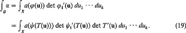
On the other hand, the change of variables theorem gives
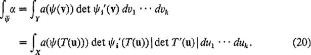
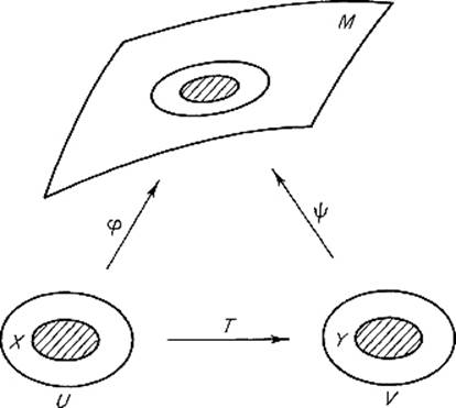
Figure 5.30
Since det T′ > 0 either if φ and ![]() are both orientation-preserving or if both are orientation-reversing, while det T′ > 0 otherwise, the conclusion of the lemma follows immediately from a comparison of formulas (19) and (20) .
are both orientation-preserving or if both are orientation-reversing, while det T′ > 0 otherwise, the conclusion of the lemma follows immediately from a comparison of formulas (19) and (20) .
![]()
Now let ![]() = {A1, . . . , Ar} and
= {A1, . . . , Ar} and ![]() = {B1, . . . , Bs} be two oriented pavings of M. Let φi and
= {B1, . . . , Bs} be two oriented pavings of M. Let φi and ![]() j be orientation-preserving parametrizations of Ai and Bj, respectively. Let
j be orientation-preserving parametrizations of Ai and Bj, respectively. Let
![]()
If φij = φi![]() Xij and
Xij and ![]() ij =
ij = ![]() j
j![]() Yij, then it follows from Lemma 5.7 that
Yij, then it follows from Lemma 5.7 that
![]()
for any k-form α defined on M. Therefore
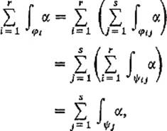
so the integral ∫M α is indeed well defined by (18) .
Integrals of differential forms on manifolds have a number of physical applications. For example, if the 2-dimensional manifold ![]() is thought of as a lamina with density function ρ, then its mass is given by the integral
is thought of as a lamina with density function ρ, then its mass is given by the integral
![]()
If M is a closed surface in ![]() 3 with unit outer normal vector field N, and F is the velocity vector field of a moving fluid in
3 with unit outer normal vector field N, and F is the velocity vector field of a moving fluid in ![]() 3., then the “flux” integral
3., then the “flux” integral
![]()
measures the rate at which the fluid is leaving the region bounded by M. We will discuss such applications as these in Section 7 .
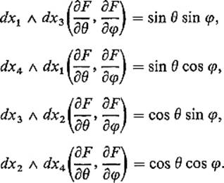
Example 6 Let T be the “flat torus” ![]() , which is the image in
, which is the image in ![]() 4 of the surface patch F : Q = [0, 2π]2 →
4 of the surface patch F : Q = [0, 2π]2 → ![]() 4 defined by
4 defined by
![]()
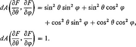
The surface area form of T is
![]()
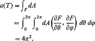
(see Exercise 5.11) . If Q is subdivided into squares Q1, Q2, Q3, Q4 as indicated in Fig. 5.31 , and Ai = φ(Qi), then {A1, A2, A3, A4} is a paving of T, so
![]()
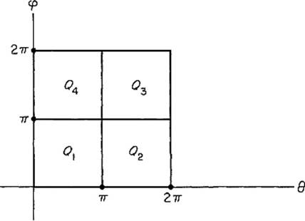
Figure 5.31
Now
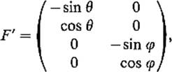
so
Therefore
Consequently
Exercises
5.1Compute the differentials of the following Compute the differentials of the following Compute the differentials of the following differential forms.
(a)Compute the differentials of the following ![]()
(b)r−nα, where r = [x12 + · · · + xn2]1/2.
(c)![]() , where (x1, . . . , xn, y1, . . . , yn) are coordinates in
, where (x1, . . . , xn, y1, . . . , yn) are coordinates in ![]() 2n
2n
5.2If F : ![]() n →
n → ![]() n is a
n is a ![]() mapping, show that
mapping, show that
![]()
5.3If ![]() is a differential 2-form on
is a differential 2-form on ![]() n, show that
n, show that
![]()
5.4The function f is called an integrating factor for the 1-form ω if f(x) ≠ 0 for all x and d(fω) = 0. If the 1-form ω has an integrating factor, show that ω ![]() dω = 0.
dω = 0.
5.5(a)If dα = 0 and dβ = 0, show that d(α ![]() β) = 0.
β) = 0.
(b)The differential form β is called exact if there exists a differential form γ such that dγ = β. If dα = 0 and β is exact, prove that α ![]() β is exact.
β is exact.
5.6Verify formula (7) in this section.
5.7If φ : Q → ![]() k is the identity (or inclusion) mapping on the k-dimensional interval
k is the identity (or inclusion) mapping on the k-dimensional interval ![]() , and α = f dx1
, and α = f dx1 ![]() · · ·
· · · ![]() dxk, show that
dxk, show that
![]()
5.8Let φ : ![]() m →
m → ![]() n be a
n be a ![]() mapping. If α is a k-form on
mapping. If α is a k-form on ![]() n, prove that
n, prove that
![]()
This fact, that the value of φ*α on the vectors v1, . . . , vk is equal to the value of α on their images under the induced linear mapping dφ, is often taken as the definition of the pullback φ*α.
5.9Let C be a smooth curve (or 1-manifold) in ![]() n, with pathlength form ds. If φ : U → C is a coordinate patch defined for
n, with pathlength form ds. If φ : U → C is a coordinate patch defined for ![]() , show that
, show that
![]()
5.10Let M be a smooth 2-manifold in ![]() n, with surface area form dA. If φ : U → M is a coordinate patch defined on the open set
n, with surface area form dA. If φ : U → M is a coordinate patch defined on the open set ![]() , show that
, show that
![]()
with E, G, F defined as in Example 5 of Section 4 .
5.11Deduce, from the definition of the surface area form, the area form of the flat torus used in Example 6.
5.12Let ![]() be an oriented smooth k-manifold with area form dA1, and
be an oriented smooth k-manifold with area form dA1, and ![]() an oriented smooth l-manifold with area form dA2. Regarding dA1 as a form on
an oriented smooth l-manifold with area form dA2. Regarding dA1 as a form on ![]() m + n which involves only the variables x1, . . . , xm, and dA2 as a form in the variables xm + 1, . . . , xm + n, show that
m + n which involves only the variables x1, . . . , xm, and dA2 as a form in the variables xm + 1, . . . , xm + n, show that
![]()
is the surface area form of the oriented (k + l)-manifold ![]() . Use this result to obtain the area form of the flat torus in
. Use this result to obtain the area form of the flat torus in ![]() 4.
4.
5.13Let M be an oriented smooth (n − 1)-dimensional manifold in ![]() n. Define a unit vector field N : M →
n. Define a unit vector field N : M → ![]() n on M as follows. Given
n on M as follows. Given ![]() , choose an orientation-preserving coordinate patch φ: U → M with x = φ(u). Then let the ith component ni(x) of N(x) be given by
, choose an orientation-preserving coordinate patch φ: U → M with x = φ(u). Then let the ith component ni(x) of N(x) be given by
![]()
(a)Show that N is orthogonal to each of the vectors ∂φ/∂u1, . . . , ∂φ/∂un−1, so N is a unit normal vector field on M.
(b)Conclude that the surface area form of M is
![]()
(c)In particular, conclude (without the use of any coordinate system) that the surface area form of the unit sphere ![]() is
is
![]()
5.14(a)If F : ![]() l →
l → ![]() m and G :
m and G : ![]() m →
m → ![]() n are
n are ![]() mappings, show that
mappings, show that
![]()
That is, if α is a k-form on ![]() n and H = G
n and H = G ![]() F then H*α = F*(G*α).
F then H*α = F*(G*α).
(b)Use Theorem 5.4 to deduce from (a) that, if φ is a k-dimensional surface patch in ![]() m, F :
m, F : ![]() m →
m → ![]() n is a
n is a ![]() mapping, and α is a k-form on
mapping, and α is a k-form on ![]() n, then
n, then
![]()
5.15Let α be a differential k-form on ![]() n. If
n. If
![]()
prove that
![]()
where A = (aij).