Advanced Calculus of Several Variables (1973)

Part VI. The Calculus of Variations

Chapter 2. CONTINUOUS LINEAR MAPPINGS AND DIFFERENTIALS

In this section we discuss the concepts of linearity, continuity, and differentiability for mappings from one normed vector space to another. The definitions here will be simply repetitions of those (in Chapters I and II) for mappings from one Euclidean space to another.

Let E and F be vector spaces. Recall that the mapping φ : E → F is called linear if

for all and .

Example 1 The real-valued function , defined on the vector space of all continuous functions on [a, b] by

is clearly a linear mapping from .

If the vector spaces E and F are normed, then we can talk about limits (of mappings from E to F). Given a mapping f : E → F and , we say that

if, given > 0, there exists δ > 0 such that

The mapping f is continuous at if

We saw in Section I.7 (Example 8) that every linear mapping between Euclidean spaces is continuous (everywhere). However, for mappings between infinite-dimensional normed vector spaces, linearity does not, in general, imply continuity.

Example 2 Let V be the vector space of all continuous real-valued functions on [0, 1], as in Example 2 of Section 1. Let E₁ denote V with the 1-norm ₁, and let E₀ denote V with the sup norm ₀. Consider the identity mapping λ : V → V as a mapping from E₁ to E₀,

We inquire as to whether λ is continuous at (the constant zero function on [0, 1 ]). If it were, then, given > 0, there would exist δ > 0 such that

However we saw in Section 1 that, given δ > 0, there exists a function φ : [0, 1 ] → such that

It follows that λ : E₁ → E₀ is not continuous at .

The following theorem provides a useful criterion for continuity of linear mappings.

Theorem 2.1 Let L : E → F be a linear mapping where E and F are normed vector spaces. Then the following three conditions on L are equivalent:

(a)There exists a number c > 0 such that

for all .

(b)L is continuous (everywhere).

(c)L is continuous at .

PROOF Suppose first that (a) holds. Then, given and > 0,

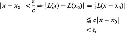
so it follows that L is continuous at x₀. Thus (a) implies (b).

To see that (c) implies (a), assume that L is continuous at 0, and choose δ > 0 such that implies L(x) < 1. Then, given , it follows that

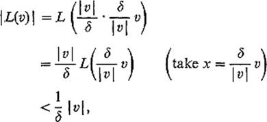
so we may take c = 1/δ.

Example 3 Let E₀ and E₁ be the normed vector spaces of Example 2, but this time consider the identity mapping on their common underlying vector space V as a linear mapping from E₀ to E₁,

Since

we see from Theorem 2.1 (with c = 1) that μ is continuous.

Thus the inverse of a one-to-one continuous linear mapping of one normed vector space onto another need not be continuous. Let L : E → F be a linear mapping which is both one-to-one and surjective (that is, L(E) = F). Then we will call L an isomorphism (of normed vector spaces) if and only if both L and L⁻¹ are continuous.

Example 4 Let A, B : [a, b] → ⁿ be continuous paths in ⁿ, and consider the linear function

defined by

where the dot denotes the usual inner product in ⁿ. Then the Cauchy-Schwarz inequality yields

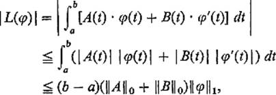
so an application of Theorem 2.1, with c = (b − a)(A₀ + B₀), shows that L is continuous.

We are now prepared to discuss differentials of mappings of normed vector spaces. The definition of differentiability, for mappings of normed vector spaces, is the same as its definition for mappings of Euclidean spaces, except that we must explicitly require the approximating linear mapping to be continuous. The mapping f : E → F is differentiable at if and only if there exists a continuous linear mapping L : E → F such that

The continuous linear mapping L, if it exists, is unique (Exercise 2.3), and it is easily verified that a linear mapping L satisfying (1) is continuous at 0 if and only if f is continuous at x (Exercise 2.4).

If f : E → F is differentiable at , then the continuous linear mapping which satisfies (1) is called the differential of f at x, and is denoted by

In the finite-dimensional case E = ⁿ, F = ^m that we are already familiar with, the m × n matrix of the linear mapping df_x is the derivative f′(x). Here we will be mainly interested in mappings between infinite-dimensional spaces, whose differential linear mappings are not representable by matrices, so derivatives will not be available.

Example 5 If f : E → F is a continuous linear mapping, then

for all with h ≠ 0, so f is differentiable at x, with df_x = f. Thus a continuous linear mapping is its own differential (at every point ).

Example 6 We now give a less trivial computation of a differential. Let g : → be a function, and define

by

We want to show that f is differentiable, and to compute its differential.

If f is differentiable at , then df_φ(h) should be the linear (in part of f(φ + h) − f(φ). To investigate this difference, we write down the second degree Taylor expansion of g at φ(t):

where

for some ξ(t) between φ(t) and φ(t) + h(t). Then

where is defined by

It is clear that is a continuous linear mapping, so in order to prove that f is differentiable at φ with df_φ = L, it suffices to prove that

Note that, since g is a function, there exists M > 0 such that g″(ξ(t)) < 2M when h₀ is sufficiently small (why?). It then follows from (2) that

and this implies (3) as desired. Thus the differential of f at φ is defined by

The chain rule for mappings of normed vector spaces takes the expected form.

Theorem 2.2 Let U and V be open subsets of the normed vector spaces E and F respectively. If the mappings f : U → F and g : V → G (a third normed vector space) are differentiable at and respectively, then their composition h = g f is differentiable at x, and

The proof is precisely the same as that of the finite-dimensional chain rule (Theorem II.3.1), and will not be repeated.

There is one case in which derivatives (rather than differentials) are important. Let φ : → E be a path in the normed vector space E. Then the familiar limit

if it exists, is the derivative or velocity vector of φ at t. It is easily verified that φ′(t) exists if and only if φ is differentiable at t, in which case dφ_t(h) = φ′(t)h (again, just as in the finite-dimensional case).

In the following sections we will be concerned with the problem of minimizing (or maximizing) a differentiable real-valued function f : E → on a subset M of the normed vector space E. In order to state the result which will play the role that Lemma II.5.1 does in finite-dimensional maximum–minimum problems, we need the concept of tangent sets. Given a subset M of the normed vector space E, the tangent set TM_x of M at the point is the set of all those vectors , for which there exists a differentiable path such that φ(0) = x and φ′(0) = v. Thus TM_x is simply the set of all velocity vectors at x of differentiable paths in M which pass through x. Hence the tangent set of an arbitrary subset of a normed vector space is the natural generalization of the tangent space of a submanifold of ⁿ.

The following theorem gives a necessary condition for local maxima or local minima (we state it for minima).

Theorem 2.3 Let the function f : E → be differentiable at the point x of the subset M of the normed vector space E. If for all sufficiently close to x, then

That is, df_x(v) = 0 for all .

PROOF Given , let φ : → M be a differentiable path in E such that φ(0) = x and φ′(0) = v. Then the composition g = f φ : → has a local minimum at 0, so g′(0) = 0. The chain rule therefore gives

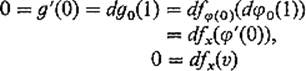
as desired.

In Section 4 we will need the implicit mapping theorem for mappings of complete normed vector spaces. Both its statement and its proof, in this more general context, are essentially the same as those of the finite-dimensional implicit mapping theorem in Chapter III.

For the statement, we need to define the partial differentials of a differentiable mapping which is defined on the product of two normed vector spaces E and F. The product set E × F is made into a vector space by defining

If _E and _F denote the norms on E and F, respectively, then

defines a norm on E × F, and E × F is complete if both E and F are (see Exercise 1.4). For instance, if E = F = with the ordinary norm (absolute value), then this definition gives the sup norm on the plane × = ²(Example 1 of Section 1).

Now let the mapping

be differentiable at the point . It follows easily (Exercise 2.5) that the mappings

defined by

are differentiable at and , respectively. Then d_xf_{(a, b)} and d_yf_{(a, b)}, the partial differentials of f at (a, b), with respect to and , respectively, are defined by

Thus d_xf_{(a, b)} is the differential of the mapping E → G obtained from f : E × F → G by fixing y = b, and d_yf_{(a, b)} is obtained similarly by holding x fixed. This generalizes our definition in Chapter III of the partial differentials of a mapping from ^m+n = ^m × ⁿ to ^k.

With this notation and terminology, the statement of the implicit mapping theorem is as follows.

Implicit Mapping Theorem Let f : E × F → G be a mapping, where E, F, and G are complete normed vector spaces. Suppose that f(a, b) = 0, and that

is an isomorphism. Then there exists a neighborhood U of a in E, a neighborhood W of (a, b) in E × F, and a mapping φ : U → F such that the following is true: If and , then f(x, y) = 0 if and only if y = φ(x).

This statement involves mappings from one normed vector space to another, whereas we have defined only differentiable ones. The mapping g : E → F of normed vector spaces is called continuously differentiable, or , if it is differentiable and dg_x(v) is a continuous function of (x, v), that is, the mapping (x, y) → dg_x(v) from E × E to F is continuous.

As previously remarked, the proof of the implicit mapping theorem in complete normed vector spaces is essentially the same as its proof in the finite-dimensional case. In particular, it follows from the inverse mapping theorem for complete normed vector spaces in exactly the same way that the finite-dimensional implicit mapping theorem follows from the finite-dimensional inverse mapping theorem (see the proof of Theorem III.3.4). The general inverse mapping theorem is identical to the finite-dimensional case (Theorem III.3.3), except that Euclidean space ⁿ is replaced by a complete normed vector space E. Moreover the proof is essentially the same, making use of the contraction mapping theorem. Finally, the only property of ⁿ that was used in the proof of contraction mapping theorem, is that it is complete. It would be instructive for the student to reread the proofs of these three theorems in Chapter III, verifying that they generalize to complete normed vector spaces.

Exercises

2.1Show that the function is continuous on .

2.2If L : ⁿ → E is a linear mapping of ⁿ into a normed vector space, show that L is continuous.

2.3Let f : E → F be differentiable at , meaning that there exists a continuous linear mapping L : E → F satisfying Eq. (1) of this section. Show that L is unique.

2.4Let f : E → F be a mapping and L : E → F a linear mapping satisfying Eq. (1). Show that L is continuous if and only if f is continuous at x.

2.5Let f : E × F → G be a differentiable mapping. Show that the restrictions φ : E → G and ψ : F → G of Eq. (4) are differentiable.

2.6If the mapping f : E × F → G is differentiable at , show that d_xf_p(r) = df_p(r, 0) and d_yf_p(s) = df_p(0, s).

2.7Let be a translate of the closed subspace V of the normed vector space E. That is, given . Then prove that TM_x = V.