Advanced Calculus of Several Variables (1973)

Part VI. The Calculus of Variations

Chapter 3. THE SIMPLEST VARIATIONAL PROBLEM

We are now prepared to discuss the first problem mentioned in the introduction to this chapter. Given f : ³ → , we seek to minimize (or maximize) the function defined by

amongst those functions such that ψ(a) = α and ψ(b) = β (where α and β are given real numbers).

Let M denote the subset of consisting of those functions ψ that satisfy the endpoint conditions ψ(a) = α and ψ(b) = β. Then we are interested in the local extrema of F on the subset M. If F is differentiable at , and FM has a local extremum at φ, then Theorem 2.3 implies that

We will say that the function is an extremal for F on M if it satisfies the necessary condition (2). We will not consider here the difficult matter of finding sufficient conditions under which an extremal actually yields a local extremum.

In order that we be able to ascertain whether a given function is or is not an extremal for F on M, that is, whether or not dF_φ TM_φ = 0, we must (under appropriate conditions on f) explicitly compute the differential dF_φ of F at φ, and we must determine just what the tangent set TM_φ of M at φ is.

The latter problem is quite easy. First pick a fixed element . Then, given any , the difference φ − φ₀ is an element of the subspace

of , consisting of those functions on [a, b] that are zero at both end-points. Conversely, if , then clearly . Thus M is a hyperplane in , namely the translate by φ₀ of the subspace . But the tangent set of a hyperplane is, at every point, simply the subspace of which it is a translate (see Exercise 2.7). Therefore

for every .

The following theorem gives the computation of dF_φ.

Theorem 3.1 Let be defined by (1), with f : ³ → being a function. Then F is differentiable with

for all .

In the use of partial derivative notation on the right-hand side of (4), we are thinking of .

PROOF If F is differentiable at , then dF_φ(h) should be the linear (in h) part of F(φ + h) − F(φ). To investigate this difference, we write down the second degree Taylor expansion of f at the point .

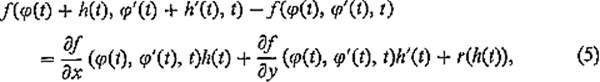
where

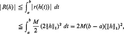
for some point ξ(t) of the line segment in ³ from (φ(t), φ′(t), t) to (φ(t) + h(t), φ′(t) + h′(t), t). If B is a large ball in ³ that contains in its interior the image of the continuous path , and M is the maximum of the absolute values of the second order partial derivatives of f at points of B, then it follows easily that

for all , if h₀ is sufficiently small.

From (5) we obtain

with

and

In order to prove that F is differentiable at φ with dF_φ = L as desired, it suffices to note that is a continuous linear function (by Example 4 of Section 2), and then to show that,

But it follows immediately from (6) that

and this implies (7).

With regard to condition (2), we are interested in the value of dF_φ(h) when .

Corollary 3.2 Assume, in addition to the hypotheses of Theorem 3.1, that φ is a function and that . Then

PROOF If φ is a function, then ∂f/∂y(φ(t), φ′(t), t) is a function of . A simple integration by parts therefore gives

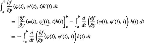
because h(a) = h(b) = 0. Thus formula (8) follows from formula (4) in this case.

This corollary shows that the function is an extremal for F on M if and only if

for every function h on [a, b] such that h(a) = h(b) = 0. The following lemma verifies the natural guess that (9) can hold for all such h only if the function within the brackets in (9) vanishes identically on [a, b].

Lemma 3.3 If φ : [a, b] → is a continuous function such that

for every , then φ is identically zero on [a, b].

PROOF Suppose, to the contrary, that φ(t₀) ≠ 0 for some . Then, by continuity, φ is nonzero on some interval containing t₀, say, φ(t) > 0 for . If h is defined on [a, b] by

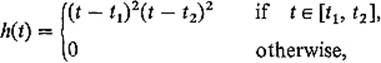
then , and

because the integrand is positive except at the endpoints t₁ and t₂ (Fig. 6.3). This contradiction proves that φ ≡ 0 on [a, b].

The fundamental necessity condition for extremals, the Euler–Lagrange equation, follows immediately from Corollary 3.2 and Lemma 3.3.

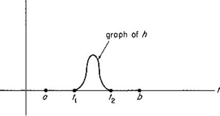
Figure 6.3

Theorem 3.4 Let be defined by (1), with f : ³ → being a function. Then the function is an extremal for F on : ψ(a) = α) and ψ(b) = β} if and only if

for all .

Equation (10) is the Euler–Lagrange equation for the extremal φ. Note that it is actually a second order (ordinary) differential equation for φ, since the chain rule gives

where the partial derivatives of f are evaluated at .

REMARKS The hypothesis in Theorem 3.4 that the extremal φ is a function (rather than merely ) is actually unnecessary. First, if φ is an extremal which is only assumed to be then, by a more careful analysis, it can still be proved that ∂f/∂y(φ(t), φ′(t), t) is a differentiable function (of t) satisfying the Euler–Lagrange equation. Second, if φ is a extremal such that

for all , then it can be proved that φ is, in fact, a function. We will not include these refinements because Theorem 3.4 as stated, with the additional hypothesis that φ is , will suffice for our purposes.

We illustrate the applications of the Euler–Lagrange equation with two standard first examples.

Example 1 We consider a special case of the problem of finding the path of minimal length joining the points (a, α) and (b, β) in the tx-plane. Suppose in particular that φ : [a, b] → is a function with φ(a) = α and φ(b) = βwhose graph has minimal length, in comparison with the graphs of all other such functions. Then φ is an extremal (subject to the endpoint conditions) of the function

whose integrand function is

Since ∂f/∂x = 0 and ∂f/∂y = y/(1 + y²)^1/2, the Euler–Lagrange equation for φ is therefore

which upon computation reduces to

Therefore φ″ = 0 on [a, b], so φ is a linear function on [a, b], and its graph is (as expected) the straight line segment from (a, α) to (b, β).

Example 2 We want to minimize the area of a surface of revolution. Suppose in particular that φ : [a, b] → is a function with φ(a) = α and φ(b) = β, such that the surface obtained by revolving the curve x = φ(t) about the t-axis has minimal area, in comparison with all other surfaces of revolution obtained in this way (subject to the endpoint conditions). Then φ is an extremal of the function

whose integrand function is

Here

Upon substituting x = φ(t), y = φ′(t) into the Euler–Lagrange equation, and simplifying, we obtain

It follows that

(differentiate the latter equation), or

The general solution of this first order equation is

where d is a second constant. Thus the curve x = φ(t) is a catenary (Fig. 6.4) passing through the given points (a, α) and (b, β).

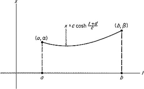
Figure 6.4

It can be shown that, if b − a is sufficiently large compared to α and β, then no catenary of the form (11) passes through the given points (a, α) and (b, β), so in this case there will not exist a smooth extremal.

This serves to emphasize the fact that the Euler–Lagrange equation merely provides a necessary condition that a given function φ maximize or minimize the given integral functional F. It may happen either that there exist no extremals (solutions of the Euler–Lagrange equation that satisfy the endpoint conditions), or that a given extremal does not maximize or minimize F (just as a critical point of a function on ⁿ need not provide a maximum or minimum).

All of our discussion thus far can be generalized from the real-valued to the vector-valued case, that is obtained by replacing the space of real-valued functions with the space of paths in ⁿ. The proofs are all essentially the same, aside from the substitution of vector notation for scalar notation, so we shall merely outline the results.

Given a function f : ⁿ × ⁿ × → , we are interested in the extrema of the function defined by

amongst those paths ψ : [a, b] → ⁿ such that ψ(a) = α and ψ(b) = β, where α and β are given points in ⁿ.

Denoting by M the subset of consisting of those paths that satisfy the endpoint conditions, the path is an extremal for F on M if and only if

We find, just as before, that M is a hyperplane. For each ,

With the notation , let us write

so ∂f/∂x and ∂f/∂y are vectors. If φ is a path in ⁿ and , then we find (by generalizing the proofs of Theorem 3.1 and Corollary 3.2) that

Compare this with Eq. (8); here the dot denotes the Euclidean inner product in ⁿ.

By an n-dimensional version of (Lemma 3.3), it follows from (13) that the path is an extremal for F on M if and only if

This is the Euler–Lagrange equation in vector form. Taking components, we obtain the scalar Euler–Lagrange equations

Example 3 Suppose that φ : [a, b] → ⁿ is a minimal-length path with endpoints α = φ(a) and β = φ(b). Then φ is an extremal for the function defined by

whose integrand function is

Since ∂f/∂x_i = 0 and ∂f/∂y_i = y_i/(y₁² + · · · + y_n²)^1/2, the Euler-Lagrange equation for φ give

Therefore the unit tangent vector φ′(t)/φ′(t) is constant, so it follows that the image of φ is the straight line segment from α to β.

Exercises

3.1Suppose that a particle of mass m moves in the force field F: ³ → ³, where F(x) = − ∇ V(x) with V: ³ → a given potential energy function. According to Hamilton's principle, the path φ : [a, b] → ³ of the particle is an extremal of the integral of the difference of the kinetic and potential energies of the particle,

Show that the Euler-Lagrange equations (15) for this problem reduce to Newton's law of motion

3.2If f(x, y, t) is actually independent of t, so ∂f/∂t = 0, and φ: [a, b] → satisfies the Euler-Lagrange equation

show that y ∂f/∂y − f is constant, that is,

for all .

3.3(The brachistochrone) Suppose a particle of mass m slides down a frictionless wire connecting two fixed points in a vertical plane (Fig. 6.5). We wish to determine the shape y = φ(x) of the wire if the time of descent is minimal. Let us take the origin as the initial point, with the y-axis pointing downward. The velocity v of the particle is determined by the energy equation , whence . The time T of descent from (0, 0) to (x₁, y₁) is therefore given by

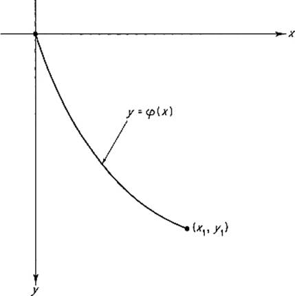
Figure 6.5

Show that the curve of minimal descent time is the cycloid

generated by the motion of a fixed point on the circumference of a circle of radius a which rolls along the x-axis [the constant a being determined by the condition that it pass through the point (x₁, y₁)]. Hint: Noting that

is independent of x, apply the result of the previous exercise,

Make the substitution y = 2a sin² θ/2 in order to integrate this equation.

Geodesics. In the following five problems we discuss geodesics (shortest paths) on a surface S in ³. Suppose that S is parametrized by , and that the curve γ : [a, b] → S is the composition γ = T c, where . Then, by Exercise V.1.8, the length of γ is

where

In order for γ to be a minimal-length path on S from γ(a) to γ(b), it must therefore be an extremal for the integral s(γ). We say that γ is a geodesic on S if it is an extremal (with endpoints fixed) for the integral

which is somewhat easier to work with.

3.4(a)Suppose that f(x₁, x₂, y₁, y₂, t) is independent of t, so ∂f/∂t = 0. If φ(t) = (x₁(t), x₂(t)) is an extremal for

prove that

is constant for . Hint: Show that

(b)If f(u, v, u′, v′) = E(u, v)(u′)² + 2F(u, v)u′v′ + G(u, v)(v′)², show that

(c)Conclude from (a) and (b) that a geodesic φ on the surface S is a constant-speed curve, φ′(t) = constant.

3.5Deduce from the previous problem [part (c)] that, if γ: [a, b] → S is a geodesic on the surface S, then γ is an extremal for the pathlength integral s(γ). Hint: Compare the Euler-Lagrange equations for the two integrals.

3.6Let S be the vertical cylinder x² + y² = r² in ³, and parametrize S by , where T(θ, z) = (r cos θ, r sin θ, z). If γ(t) = T(θ(t), z(t)) is a geodesic on S, show that the Euler-Lagrange equations for the integral (*) reduce to

so θ(t) = at + b, z(t) = ct + d. The case a = 0 gives a vertical straight line, the case c = 0 gives a horizontal circle, while the case a ≠ 0, c ≠ 0 gives a helix on S (see Exercise II.1.12).

3.7Generalize the preceding problem to the case of a “generalized cylinder” which consists of all vertical straight lines through the smooth curve .

3.8Show that the geodesics on a sphere S are the great circles on S.

3.9Denote by the vector space of twice continuously differentiable functions on [a, b], and by the subspace consisting of those functions such that ψ(a) = ψ′(a) = ψ(b) = ψ′(b) = 0.

(a)Show that

defines a norm on .

(b)Given a function f: ⁴ → , define by

Then prove, by the method of proof of Theorem 3.1, that F is differentiable with

where the partial derivatives of f are evaluated at (φ(t), φ′(t), φ″(t), t).

(c)Show, by integration by parts as in the proof of Corollary 3.2, that

if .

(d)Conclude that φ satisfies the second order Euler-Lagrange equation

if φ is an extremal for F, subject to given endpoint conditions on φ and φ′ (assuming that φ is of class —note that the above equation is a fourth order ordinary differential equation in φ).