Advanced Calculus of Several Variables (1973)

Part VI. The Calculus of Variations

Chapter 5. MULTIPLE INTEGRAL PROBLEMS

Thus far, we have confined our attention to extremum problems associated with the simple integral , where is a function of one variable. In this section we briefly discuss the analogous problems associated with a multiple integral whose integrand involves an “unknown” function of several variables.

Let D be a cellulated n-dimensional region in ⁿ. Given f : ²ⁿ⁺¹ → , we seek to maximize or minimize the function F defined by

amongst those functions : D → which agree with a given fixed function ₀ : D → on the boundary ∂D of the region D. In terms of the gradient vector

we may rewrite (1) as

Throughout this section we will denote the first n coordinates in ²ⁿ⁺¹ by x₁, . . . , x_n, the (n + 1)th coordinate by y, and the last n coordinates in ²ⁿ⁺¹ by z₁, . . . , z_n. Thus we are thinking of the Cartesian factorization ²ⁿ⁺¹ = ⁿ × × ⁿ, and therefore write (x, y, z) for the typical point of ²ⁿ⁺¹. In terms of this notation, we are interested in the function

where y = ψ(x) and z = ∇(x).

The function F is defined by (2) on the vector space that consists of all real-valued functions on D (with the usual pointwise addition and scalar multiplication). We make into a normed vector space by defining

It can then be verified that the normed vector space is complete. The proof of this fact is similar to that of Corollary 1.5 (that is complete), but is somewhat more tedious, and will be omitted (being unnecessary for what follows in this section).

Let M denote the subset of consisting of those functions that satisfy the “boundary condition”

Then, given any , the difference ψ − ψ₀ is an element of the subspace

of , consisting of all those functions on D that vanish on ∂D. Conversely, if , then clearly . Thus M is a hyperplane in , namely, the translate by the fixed element of the subspace . Consequently

for all .

If is differentiable at , and FM has a local extremum at φ, Theorem 2.3 implies that

Just as in the single-variable case, we will call the function an extremal for F on M if it satisfies the necessary condition (4).

The following theorem is analogous to Theorem 3.1, and gives the computation of the differential dF_φ when F is defined by (1).

Theorem 5.1 Suppose that D is a compact cellulated n-dimensional region in ⁿ, and that f : ²ⁿ⁺¹ → is a function. Then the function defined by (1) is differentiable with

for all . The partial derivatives

in (5) are evaluated at the point .

The method of proof of Theorem 5.1 is the same as that of Theorem 3.1, making use of the second degree Taylor expansion of f. The details will be left to the reader.

In view of condition (4), we are interested in the value of dF_φ(h) when . The following theorem is analogous to Corollary 3.2.

Theorem 5.2 Assume, in addition to the hypotheses of Theorem 5.1, that φ is a function and that . Then

Here also the partial derivatives of f are evaluated at .

PROOF Consider the differential (n − 1)-form defined on D by

A routine computation gives

where dx = dx₁ · · · dx_n. Hence

Substituting this into Eq. (5), we obtain

But ∫_D dω = ∫_∂D ω = 0 by Stokes' theorem and the fact that ω = 0 on ∂D because . Thus Eq. (7) reduces to the desired Eq. (6).

Theorem 5.2 shows that the function is an extremal for F on M if and only if

for every . From this result and the obvious multivariable analog of Lemma 3.3 we immediately obtain the multivariable Euler–Lagrange equation.

Theorem 5.3 Let be defined by Eq. (1), with f : ²ⁿ⁺¹ → being a function. Then the function is an extremal for F on M if and only if

for all .

The equation

with the partial derivatives of f evaluated at (x, φ(x), ∇φ(x)), is the Euler–Lagrange equation for the extremal φ. We give some examples to illustrate its applications.

Example 1 (minimal surfaces) If D is a disk in the plane, and φ₀ : D → a function, then the graph of φ₀ is a disk in ³. We consider the following question. Under what conditions does the graph (Fig. 6.8) of the function φ : D → have minimal surface area, among the graphs of all those functions : D → that agree with φ₀ on the boundary curve ∂D of the disk D?

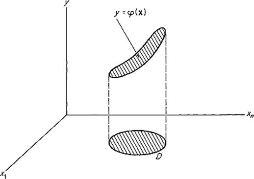
Figure 6.8

We can just as easily discuss the n-dimensional generalization of this question. So we start with a smooth compact n-manifold-with-boundary , and a function φ₀ : D → , whose graph y = φ₀(x) is an n-manifold-with-boundary in ^{n + 1}.

The area F(φ) of the graph of the function φ : D → is given by formula (10) of Section V.4,

We therefore want to minimize the function defined by (1) with

Since

the Euler–Lagrange equation (8) for this problem is

Upon calculating the indicated partial derivatives and simplifying, we obtain

where

as usual. Equation (9) therefore gives a necessary condition that the area of the graph of y = φ(x) be minimal, among all n-manifolds-with-boundary in ⁿ⁺¹ that have the same boundary.

In the original problem of 2-dimensional minimal surfaces, it is customary to use the notation

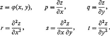
With this notation, Eq. (9) takes the form

This is of course a second order partial differential equation for the unknown function z = φ(x, y).

Example 2 (vibrating membrane) In this example we apply Hamilton's principle to derive the wave equation for the motion of a vibrating n-dimensional “membrane.” The cases n = 1 and n = 2 correspond to a vibrating string and an “actual” membrane, respectively.

We assume that the equilibrium position of the membrane is the compact n-manifold-with-boundary

and that it vibrates with its boundary fixed. Let its motion be described by the function

in the sense that the graph y = φ(x, t) is the position in ⁿ⁺¹ of the membrane at time t (Fig. 6.9).

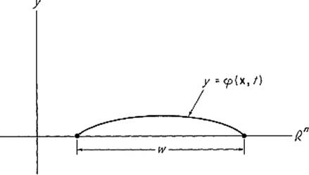
Figure 6.9

If the membrane has constant density σ, then its kinetic energy at time t is

We assume initially that the potential energy V of the membrane is proportional to the increase in its surface area, that is,

where a(t) is the area of the membrane at time t. The constant τ is called the “surface tension.” By formula (10) of Section V.4 we then have

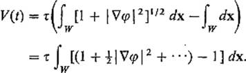
We now suppose that the deformation of the membrane is so slight that the higher order terms (indicated by the dots) may be neglected. The potential energy of the membrane at time t is then given by

According to Hamilton's principle of physics, the motion of the membrane is such that the value of the integral

is minimal for every time interval [a, b]. That is, if D = W × [a, b], then the actual motion φ is an extremal for the function defined by

on the hyperplane consisting of those functions that agree with φ on ∂D.

If we temporarily write t = x_n+1 and define f on ²ⁿ⁺³ = ²ⁿ⁺¹ × × ²ⁿ⁺¹ by

then we may rewrite (12) as

where y = ψ(x) and z = ∇(x). Since

it follows that the Euler–Lagrange equation (8) for this problem is

or

Equation (13) is the n-dimensional wave equation.