High School Algebra II Unlocked (2016)

Lesson 8.6. Confidence Intervals and Margins of Error

In many studies and experiments, the true population proportion, p, and standard deviation, σ, are unknown. In these cases, we use the sample proportion, , to approximate p. We also use the same formula we would for calculating standard deviation but substitute for p. This sample standard deviation is called the standard error.

The standard error for a sample proportion distribution is given by the formula SE = 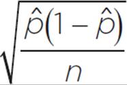, where is the sample proportion and n is the sample size.

A standard error functions like a standard deviation in interpretations of normal data distributions. For example, 68% of data lies within one SE of the sample mean, 95% lies within two SE, and 99.7% lies within three SE. However, because we do not know the true population proportion, p, these percentages instead tell us how likely p is to fall within these ranges of our value. In terms of quantities (np or n) instead of proportions, we use the standard error to determine whether the true mean of the number of successes is likely to fall within certain ranges of the sample mean, μ, of numbers of successes. These ranges are called confidence intervals.

Compare this to
the formula for the
standard deviation
of the sampling
distribution, shown
in Lesson 8.5.

For our purposes, a confidence interval is an interval that is likely to contain the population mean, to the specified level of confidence. The most common confidence levels used are 0.90, 0.95, and 0.99.

The correlation of ±2 standard errors or ±2 standard deviations to 95% is a rounded value. To be more precise, 95% of the population is within 1.96σ or 1.96SE of the mean.

A confidence interval
is an interval that is
likely, to the specified
confidence level,
to contain some
population parameter
of interest. This
could be some other
parameter, such as the
standard deviation,
rather than the mean.
Here, however, we
will only look at
confidence intervals
for population means.

The margin of error is the distance from the sample mean that is likely to include the population mean, to the desired confidence level. So, the margin of error is half the width of the confidence interval for a given confidence level.

The margin of error is often expressed using the ± symbol. For example, a report may say, “The liquid’s pH is 5.21 ± 0.05,” to indicate that the pH measure is very likely in the range between 5.16 and 5.26.

Dunja wants to estimate the number of people who will vote for the Democratic candidate for mayor in her town’s next election. She surveys a random sample of 180 people, 117 of whom said that they would vote for the Democratic candidate. There are typically about 20,000 people who vote in the town’s mayoral elections. What is the confidence interval for the number of votes the Democratic candidate will actually receive, at a 68% confidence level? What is the confidence interval for the number of votes the Democratic candidate will actually receive, at a 95% confidence level? Express each of these using the margin of error. If Dunja surveyed an additional 320 people, with the same sample proportion result, how would that affect the margin of error for a 95% confidence level?

The true proportion of people who will vote for the Democratic candidate is unknown, but the sample proportion is 117/180, or 0.65. Clearly, 0.65(20,000) ≥ 10 and (1 − 0.65)(20,000) ≥ 10, so we can use a normal distribution model.

SE = 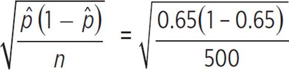≈ 0.036

We are using rounded
values, because the SE
cannot be calculated
with much precision
for a small sample size.

The sample mean, µ, is 0.65, and the standard error, SE, is 0.036. A total of 68% of possible success ratios (percents of people voting for the Democratic candidate) should be within one SE of the sample mean.

0.65 − 0.036 = 0.614
0.65 + 0.036 = 0.686

For a 68% confidence level, the confidence interval is from 0.614 to 0.686. In other words, there is a 68% probability that the Democratic candidate will receive between 61.4 and 68.6 percent of the votes. The margin of error for the proportion is one SE, or 0.036. So, for a 68% confidence level, the Democratic candidate will receive 65% of the votes plus or minus 3.6 percentage points.

The margin of error
is expressed in the
units of the standard
variable. Because we
define the sample
mean as 65 percent,
the standard error is
in percentage points.
Just as we multiplied
0.65 by 100 to convert
it to a percent, we
must also multiply
0.036 by 100.

A total of 95% of possible voting ratios should be within 1.96SE of the mean.

0.65 − 1.96(0.036) ≈ 0.579
0.65 + 1.96(0.036) ≈ 0.721

For a 95% confidence level, the confidence interval is from 0.579 to 0.721. In other words, there is a 95% probability that the Democratic candidate will receive between 57.9 and 72.1 percent of the votes. The margin of error, in this case, is 1.96(0.36) ≈ 0.071. So, for a 95% confidence level, the Democratic candidate will receive 65% of the votes plus or minus 7.1 percentage points.

If Dunja surveyed an additional 320 people, with the same proportion result of 0.65, then she will have surveyed a total of 180 + 320 = 500 people, 65% of whom said that they would vote for the Democratic candidate. We must recalculate the SE for this adjusted sample size.

SE = 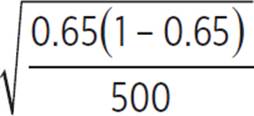≈ 0.021

For a 95% confidence level, the margin of error is now 1.96(0.021) ≈ 0.041. The margin of error has decreased, from about 0.07 for the 180-person sample, to about 0.04 for the 500-person sample. For this 500-person sample, there is a 95% chance that the Democratic candidate will receive 65% of the votes plus or minus 4.1 percentage points.

Here is how you may see margins of error on the SAT.

Bit Bikes Inc. conducted a random survey of 3,500 bike owners from around the United States. 420 of the respondents stated that they own youth bikes, while the remainder stated that they own adult bikes. After analyzing the results, Bit Bikes Inc. determines that the survey results have a margin of error of 2%. Which of the following best represents the range for the percentage of the nation’s bike owners who own adult bikes?

A) 10−14%

B) 12−16%

C) 81−85%

D) 86−90%

If Dunja wanted to estimate the actual number of people who will vote for the Democratic candidate, rather than what percent will vote for him, she would apply all percentages to the actual population of 20,000 voters.

The problem with
converting the
percentages to actual
numbers of voters
is that the 20,000
voter population is an
estimate, probably
with a great deal of
variability. The more
useful statistics are
the likely percentages
of votes that the
candidate will receive.

According to her 180-person sample, there is a 68% probability that the Democratic candidate will receive 13,000 votes ± 720 votes. According to the same sample, there is a 95% probability that the Democratic candidate will receive 13,000 votes ± 1420 votes. According to the complete 500-person survey, there is a 95% probability that the Democratic candidate will receive 13,000 votes ± 820 votes.

For a given data set, as the confidence level increases, the corresponding confidence interval also must increase, which means that the margin of error increases. Viewed in the other direction, a decrease in the margin of error requires a decrease in the confidence level for the data set.

However, an increase in sample size will decrease the margin of error without reducing the confidence level, provided that outcomes for the larger sample remain relatively consistent with the original sample.

Dave is concerned that he may have a certain medical condition, which exists in 3% of the population. He takes a diagnostics test that indicates that he does have the condition. For people who truly have the condition, this diagnostics test correctly diagnoses them with an 82% confidence level, meaning that it produces false negative results 18% of the time. For people who do not actually have the condition, this diagnostics test correctly diagnoses them with a 90% confidence level, meaning that it produces false positive results 10% of the time.

The probability, based on his test results, that Dave truly does have the condition is the ratio of true positive results to total positive results (both true and false) that the diagnostics test would produce for the population.

Treatment for this condition is expensive and involves potentially serious side effects, so Dave only wants to get treatment if his probability of actually having the condition is greater than 25%. Should Dave seek treatment?

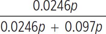
If we define p to be the total number of people in the population, then the number of people who actually have the medical condition is 0.03p (3% of p). Of these 0.03p people, 82% would be correctly diagnosed using this test, for a total of 0.82(0.03p) = 0.0246p true positive results.

Because 3% of the population has the condition, the other 97% does not. The number of people who do not have the condition is 0.97p. Of these people, 10% will get incorrectly diagnosed as having the condition. This means a total of 0.1(0.97p) = 0.097pfalse positive results.

Probability Dave has the condition =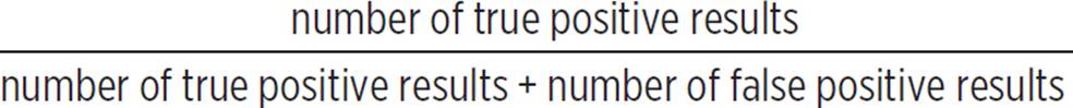

=

=

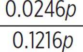
= 0.0246/0.1216

≈ 0.20

The probability that Dave actually has this medical condition is about 20%, which is less than 25%. According to his conditional statement, he should not seek treatment.

According to survey results, 420 of 3500 bike owners own youth bikes, so 3500 − 420 = 3080 own adult bikes. As a percentage of bike owners surveyed, this is 3080/3500 = 0.88, or 88%. Based on these survey results, about 88% of bike owners in the United States own adult bikes.

The margin of error is 2 percentage points, so the actual percentage of bike owners in the United States who own adult bikes is highly likely be between 88 − 2 and 88 + 2 percent, or between 86% and 90%. The correct answer is (D).

DRILL

CHAPTER 8 PRACTICE QUESTIONS

Click here to download a PDF of Chapter 8 Practice Questions.

Directions: Complete the following open-ended problems as specified by each question stem. For extra practice after answering each question, try using an alternative method to solve the problem or check your work.

1. A school has to eliminate some of its extracurricular activities. It surveys a randomly selected group of 100 of the 2500 students in the school, providing options of four extracurricular activities and allowing each student to choose just one to nominate for elimination. The survey finds that of the 100 students surveyed, 42 think that band should be eliminated, 24 think that chorus should be eliminated, 18 think that the golf team should be eliminated, and 16 think that the cooking club should be eliminated.

(a) Given this survey, how many students in the school likely believe that the school should eliminate each of the four activities?

(b) The principal decides to eliminate three out of the four extracurricular activities mentioned on the survey. Based on the survey results, she concludes that most students in the school want to keep the cooking club. What is the flaw in her reasoning? How should she redesign the survey if she wants to choose three activities to eliminate based on the one activity the most students want to keep?

2. A bowler in a tournament bowls 8 games and gets scores of 190, 255, 210, 160, 173, 188, 206, and 224.

(a) Determine the mean, range, and interquartile range of her scores. Also calculate the variance and standard deviation for the set.

(b) Suppose that this is a representative sample of the 250 games this bowler has played this year. What is the estimated standard deviation of her scores for the year? A total of 68% of her scores are likely to fall within what range of scores? Express this as a number of games.

3. A student is conducting a survey for her Psychology class. She has heard that there is a correlation between the color of a jersey a team wears and the perceived aggressiveness of the team; for example, a team that wears black jerseys is perceived as more aggressive than one wearing white jerseys.

(a) She wants to conduct a survey in her school to see who agrees with this notion. Her first thought is to just ask everyone in all of her classes, giving a survey to each person that shares a class with her. Her second idea is to ask her teachers to give them out to all students in their classes each day. What is wrong with each of these methods, and what method could she use instead to ensure she gets survey responses from a representative sample of schoolmates?

(b) What are the problems with using a survey to study this correlation? How might a scientist design an experiment to study the correlation with less bias?

4. Describe the type of probability distribution for each of the following:

(a) the theoretical probabilities of Lillian choosing each of her seven scarves if she randomly chooses one to wear

(b) the set of possible experimental probabilities of Lillian choosing her blue scarf if randomly choosing one to wear each day

(c) the probabilities that an adult alligator chosen at random will measure any given length

(d) the probabilities that an alligator chosen at random from a group of 50 adults and 50 one-week-olds (not previously measured) will measure any given length

5. A movie theater surveys its patrons regarding its pricing for food and beverage. Of the 1200 people who visited the theater on a given day, 1056 of them said they would not pay more than $15.00 for a combo that included a large drink and a large popcorn. The theater determines that there is a margin of error of 18 patrons for a 68% confidence level for an extrapolation of these survey results to the full population of their patrons. For a 95% confidence level, what is the likely percentage range for the moviegoers who would not purchase the combo at a price more than $15.00?

6. A teacher sets her scoring curve along a normal distribution curve based on the results of a given test. On this particular test, 68% of the students scored between a 56 and an 82. In order to pass the test, the teacher requires a student to have achieved more than the mean score. In order to get an A, the student must be in the 95^th percentile, and to get an A+ on the test, a student must achieve a score greater than three standard deviations above the mean. What score would be needed to pass? To get an A? To get an A+?

7. A popular television show ran for 10 seasons, with a total of 236 episodes. Now, a certain channel shows seemingly randomly chosen episodes of this show as reruns, with 2 episodes per night, 5 nights per week, for a total of 10 episodes per week. In the past 20 weeks, there has never been a repeat of the same episode within a given week. (For our purposes, define a given week as Sunday through Saturday.) Based on this information, is the selection of episodes likely to be truly random? Use statistics to support your conclusion.

8. A factory uses quality control tests for flashlights they produce. The tests correctly identify defective flashlights 80% of the time and correctly identify flashlights in perfect working condition 90% of the time. Long-term data suggests that 5% of all flashlights this factory produces are actually defective. The factory discards all flashlights labeled as defective by their quality control tests and sells the rest.

(a) Out of a batch of 10,000 flashlights, how many will the factory discard? What is the probability that a consumer purchasing a flashlight made in this factory gets a defective one?

(b) The factory makes a profit of $12 per flashlight, so they lose this amount of potential profit per properly working flashlight that they discard. The CEO is considering improving the quality control tests. For a cost of $8,000 per batch of 10,000 flashlights, the improved tests would cut the number of false positive and false negative results each in half. Is it worth it to pay for the improved quality control tests, from a cost perspective?

SOLUTIONS TO CHAPTER 8 PRACTICE QUESTIONS

1. (a) Band: 1050, Chorus: 600, Golf: 450, Cooking Club: 400; (b) See reasoning below.

(a) Set up a proportion using the sample data. Of the students surveyed, 42/100 believe band should be eliminated, 24/100 believe chorus should be eliminated, 18/100 think the golf team should be eliminated, and 16/100 say the cooking club should be eliminated. Set each of these fractions equal to an unknown number x over 2500, the actual number of students in the school. Cross-multiply and solve for x in each of the resulting proportions.

Band: 42/100 = x/2500, so x = 1050 people
Chorus: 24/100 = x/2500, so x = 600 people.
Golf: 18/100 = x/2500, so x = 450 people.
Cooking Club: 16/100 = x/2500, so x = 400 people.

Therefore, based on this sample, 1050 people would believe band should be eliminated, 600 believe chorus should be eliminated, 450 believe the golf team should be eliminated, and 400 believe the cooking club should be eliminated.

(b) The principal assumes that the extracurricular activity that the fewest students vote to eliminate is the one that the most students want to preserve, which is not necessarily the case. There are four different activities to choose from, and some may be more polarizing than others in terms of how students feel about them. It’s possible that the majority of the 84 students who voted to eliminate one of the other three activities besides the cooking club would also prefer to preserve a different one of those three activities, over the cooking club. The principal should redesign the survey to ask which extracurricular activity each student would most like to preserve and, based on the results, keep the most popular and eliminate the other three activities.

2. (a) Mean: 200.75, Range: 95, Interquartile Range: 36.5, Variance: 788.1875, Standard Deviation: 28.07; (b) Estimated Standard Deviation: 30.01, 68% of Scores Within 171 and 231, for 170 games.

(a) First, calculate the mean by adding all the scores together and dividing by the 8 games bowled. The total would be 190 + 255 + 210 + 160 + 173 + 188 + 206 + 224 = 1606 total pins, so the mean would be 1606/800 = 200.75. The range is the difference between the highest and lowest scores, so that would be 255 − 160 = 95. For the interquartile range, first reorder the numbers; the new order, from least to greatest, would be 160, 173, 188, 190, 206, 210, 224, and 255. The interquartile range is the difference between the upper quartile and lower quartile of the data set. The upper quartile is the median of the upper half of the set, {206, 210, 224, 255}, or = 217. The lower quartile is the median of the lower half of the set, {160, 173, 188, 190}, or = 180.5. The interquartile range is 217 − 180.5 = 36.5.

To calculate the variance, determine how much each of the given scores deviates from the mean using the variance equation. The result would be the following:

This simplifies as 6305.5/8, or 788.1875, so that is the variance. The standard deviation would be the square root of this number, which is 28.07.

(b) If these 8 scores are a representative sample of a total of 250 scores, then we must calculate the estimated standard deviation for the 250 scores, based on this sample. The formula for estimated standard deviation is the same as for standard deviation, except that the sum of squared differences is divided by (n − 1) instead of n.

≈ 30.01

Assuming the bowler’s scores follow a normal distribution, 68% of these scores will be within one standard deviation of her mean score. We must use the estimated standard deviation, rounded off to 30, and the mean, rounded off to 201. (Bowling scores are whole numbers.)

201 − 30 = 171
201 + 30 = 231

So, 68% of her scores are likely to be between 171 and 231. Out of 250 total games, 68% is 0.68(250) = 170. Out of the bowler’s 250 games played this year, about 170 games should have scores between 171 and 231.

3. See explanations below.

(a) If she only surveys those in her class, the results may be skewed based on shared characteristics among those in her own grade level, with her own academic interests, and/or at the same academic level (such as in honors classes). If she asks only her own teachers to give the surveys out to all students in their classes, likewise, the results will be skewed. If she is trying to conduct a survey in the school to see who agrees with the notion, she needs to ensure she surveys a representative and random population of students in the school. Therefore, she could, for example, give the survey out at lunch to random people in the cafeteria. If she wants the teachers to help, she could also pick a subject that all students must take and give a stack of the surveys to each teacher for that subject —for example, give every English teacher 10 surveys to have students fill out. Every teacher could distribute the surveys randomly to students in one of their classes, ensuring that a solid random cross-section of the school as a whole is surveyed.

(b) A survey asks people to recognize and represent their own perceptions, but they may not be consciously aware of how color affects their perceptions of aggressiveness. This introduces a bias. To study the correlation with less bias, a scientist could edit a video of two teams playing a game, so that the jerseys for one team appear as all black, all white, or all another color in each of the edited versions of the video. These versions of the same video clip, with different color jerseys, could be shown to a large sample population, with each subject asked to rate the aggressiveness of the given team on a scale of 1 to 10. The results will show whether the same team, behaving the same way, is perceived as more or less aggressive based only on the color of their jerseys, the isolated factor in the experiment.

4. (a) 1/7, (b) 0 to 1, (c) a continuous normal distribution, (d) bimodal probability distribution

(a) The theoretical probability of Lillian choosing any one of her seven scarves is 1/7, because they each have an equal chance of being randomly chosen. Each probability is the same, and there are exactly 7 distinct options, so this is an example of a discrete uniform probability distribution.

(b) Possible experimental probabilities of Lillian randomly choosing her blue scarf range from 0 to 1, but these experimental probabilities are not equally likely. Experimental probabilities close to 1/7 are likely, while experimental probabilities close to 0 or 1 are less likely. The experimental probabilities should follow a continuous normal distribution curve with a mean of 1/7, especially for a large sample space (many samples of sets of days of choosing one scarf each day). For a smaller sample space, there will be a greater standard deviation, which may result in a skewed distribution, because 1/7 is much closer to 0 than to 1.

(c) Lengths of adult alligators are probably normally distributed, because many biological measurements are. So, the probability distribution curve for weights of an adult alligator chosen at random should be a continuous normal distribution.

(d) In a group of 50 adult alligators and 50 one-week-old alligators, the frequencies of lengths should be highest around the average length of an adult alligator and the average length of a one-week-old alligator. These lengths are very different. So, the probabilities of lengths for an alligator chosen at random from such a group of 100 alligators follow a bimodal probability distribution.

5. 85 to 91%

The margin of error is 18 for a 68% confidence level, so there is a 68% probability that between 1056 − 18 and 1056 + 18 out of 1200 moviegoers are unwilling to pay more than $15.00 for the combo. The margin of error of 18 is like a standard error, or standard deviation, for a normal distribution. To find the margin of error for a 95% confidence level, we must find 1.96 times 18.

1.96 ⋅ 18 = 35.28

Out of 1200 moviegoers, there is a 95% chance that between 1056 − 35.28 and 1056 + 35.28 will be unwilling to pay more than $15.00 for the combo. We must convert these values into percentages of the total number of moviegoers.

= 0.8506

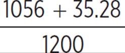= 0.9094

For a 95% confidence level, between 85 and 91 percent of moviegoers will be unwilling to pay more than $15.00 for the combo of a large drink and a large popcorn.

6. above a 68 to pass, at least 95 for an A, and at least 108 for an A+

Since the teacher sets the scoring curve along a normal distribution with 68% of the students falling between a 56 and an 82, the mean score on the test is the midpoint of this range. The middle of the range from 56 to 82 is 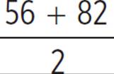, or 69; therefore, in order to pass, the student must get a score higher than a 69 on the test. If the mean score is 69, and one standard deviation from this number was 56 or 82, then the standard deviation must be 82 − 69 = 13. Since a normal distribution curve results in 95% of the scores being within two standard deviations from the mean, going up another 13 would give this point; 82 + 13 = 95, so to get an A on the test the student needs at least a 95. Three standard deviations in this case would bring the needed number up to 95 + 13 = 108, so in order to get an A+, the student would need to get a 108 on the test.

7. No, the selection is probably not truly random.

First, find the probability that there is no repeat of an episode within a given week. By the fundamental counting principle, the total number of possible sets of 10 episodes, allowing for repeats, is 236 ⋅ 236 ⋅ 236 ⋅ 236 ⋅ 236 ⋅ 236 ⋅ 236 ⋅236 ⋅ 236 ⋅ 236, or 236¹⁰. The total number of possible sets of 10 episodes without any repeats is 236 ⋅ 235 ⋅ 234 ⋅ 233 ⋅ 232 ⋅ 231 ⋅ 230 ⋅ 229 ⋅ 228 ⋅ 227. (This can also be written as the permutation 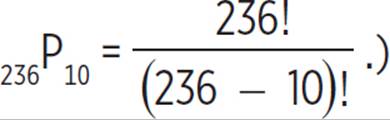The probability that the 10 episodes shown in a given week includes no repeats is , which equals approximately 0.824.

Because the probability of no repeats within the 10 episodes is 82.4%, the probability of one or more repeats is 17.6%.

We want to determine the likeliness of zero repeats per experiment (week) in a sample set of 20 experiments (20 weeks of 10 episodes being randomly selected from 236 episodes). It may be easiest to view as comparing the sample proportion (experimental probability) of 0 to the theoretical probability of having a repeat within one of the 20 weeks.

The population proportion, p, is the same as the theoretical probability of a given week including a repeated episode, 0.176. Because we are only interested in whether or not a given week includes a repeated episode, this is a Bernoulli trial. The population size, 236¹⁰, is far more than 20 times the sample size of 20, so sample proportions should be normally distributed, with a mean of 0.176 and a standard deviation of 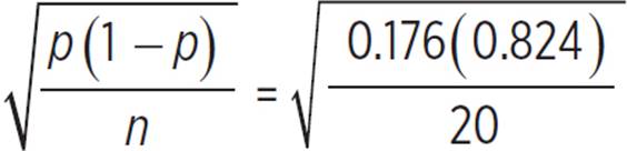, or about 0.085.

One standard deviation equals 0.085, so two standard deviations equal 0.170. A sample proportion of 0 is more than two standard deviations (0.170) less than the mean (0.176). The area under the normal distribution curve to the left of two standard deviations to the left of the mean contains half of 5% of the area under the entire curve. So, the probability of a sample proportion of 0 (0 weeks with repeats out of 20 weeks) is less than 2.5%. It seems very unlikely that there would be no episode repeats within any of the 20 weeks by chance alone. The television channel probably does not use a completely random selection method to choose episodes to air each week.

8. (a) 400, 1%; (b) No, the quality control tests would have to cost less than $5,700 for it to be worth it.

(a) Out of 10,000 flashlights produced, 5%, or 500 flashlights, will be defective, and the other 95%, or 9500, will be in perfect working condition. Of the 500 defective flashlights, 80% will be correctly identified by the quality control tests as defective.

0.80 ⋅ 500 = 400

Of the 500 defective flashlights, 400 will be identified as defective and discarded. The other 100 defective flashlights will be sold.

Of the 9500 properly working flashlights, 90% will be correctly identified as such.

0.90 ⋅ 9500 = 8550

Of the 9500 properly working flashlights, 8550 will be sold, and the other 950 will be incorrectly identified as defective and discarded.

Out of a batch of 10,000 flashlights, the factory will discard a total of 400 + 950 = 1350 flashlights. They will sell the remaining 8650. Of those 8650 flashlights, 100 are actually defective, so the probability that a consumer purchasing a flashlight made in this factory gets a defective one is 100/8650 ≈ 0.01, or about 1%.

(b) The factory loses $12 in potential profit per working flashlight they discard. They currently discard 950 working flashlights incorrectly identified as defective (a false positive) out of a batch of 10,000. If the improved quality control tests cut the number of false positives in half, then they would result in only 1/2 (950) = 475 working flashlights being discarded.

For a batch of 10,000 flashlights, the number of flashlights saved from incorrect disposal by the test improvement would be 950 − 475 = 475. The amount of money saved, in terms of potential profit, would be 475 ⋅ $12 = $5,700. However, for the improved tests, there would be a cost to the company of $8,000 per batch of 10,000 flashlights. The cost would be greater than the profits saved, so the quality control test upgrades would not be worthwhile—unless the reduction in the number of defective flashlights they sell also has a substantial positive impact on their profits.

REFLECT

Congratulations on completing Chapter 8! Here’s what we just covered. Rate your confidence in your ability to

• Understand the difference between sample surveys, experiments, and observational studies, and identify methods that provide representative sample populations for each of these

1 2 3 4 5

• Find the standard deviation or estimated standard deviation, as appropriate, for a data set, and understand the relationship between standard deviations, mean, and the normal distribution curve

1 2 3 4 5

• Use proportional reasoning, given ratios in a large representative sample population, to make inferences about the target population

1 2 3 4 5

• Understand the difference between discrete uniform, continuous uniform, normal, skewed, and bimodal probability distributions

1 2 3 4 5

• Use area under a continuous probability distribution curve, either uniform or normal, to calculate probabilities, when appropriate to the situation

1 2 3 4 5

• Use simulations to assess how well experimental results match a given model and to determine when results are statistically significant

1 2 3 4 5

• Calculate the confidence interval and margin of error for a given sample proportion at various confidence levels and for various sample sizes

1 2 3 4 5

• Use statistics and probability concepts to interpret and evaluate given statements and to analyze options in real-world situations

1 2 3 4 5

If you rated any of these topics lower than you’d like, consider reviewing the corresponding lesson before moving on, especially if you found yourself unable to correctly answer one of the related end-of-chapter questions.

Access your online student tools for a handy, printable list of Key Points for this chapter. These can be helpful for retaining what you’ve learned as you continue to explore these topics.