Idiot's Guides: Algebra I (2015)

Part V. Radical, Quadratic, and Rational Functions

Chapter 18. Rational Equations and Functions

In This Chapter

·  Solving rational equations by cross-multiplying

·  Multiplying through to clear denominators

·  Graphing rational functions

Algebra begins with variables, which quickly combine into expressions and then equations and inequalities. We started by solving linear equations, and then explored equations that involved radicals and others that involved squares. Those quadratic equations were built from polynomials and our most recent bit of building was assembling polynomials into rational expressions. Now it’s time to look at equations and functions built from rational expressions.

In this chapter, we’ll investigate the two most common ways to solve equations involving rational expressions, and we’ll explore the characteristics of the graphs of rational functions. As always, we’ll look for shortcuts, and make good use of skills we’ve already built, like factoring and operations with polynomials.

Solving Rational Equations

An equation that contains one or more rational expressions is called a rational equation. When solving rational expressions, you need to be aware of the domain of the equation. Each rational expression has a domain, a set of all the real numbers that could be substituted for the variable without making the denominator equal zero. The expression has a domain of all real numbers except 3, and the expression has a domain of all real numbers except 1 and -1. If we build a rational equation that includes both of those expressions, such as 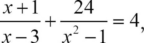the domain of the equation can’t include 3, because 3 is not in the domain of and can’t include 1 or -1, because they’re not in the domain of . The domain of the equation is all real numbers except -1, 1, and 3.

DEFINITION

A rational equation is an equation that contains one or more rational expressions.

You need to be aware of the domain of a rational equation whenever you set out to find its solution. Rational equations may have more than one solution, or one solution, or no solutions. Whenever you solve rational equations, however, you have to be alert to the possibility of an extraneous solution, and checking your solutions will be crucial.

A rational equation may be as simple as , which you can probably guess has a solution of x = 2, but they can get quite complicated. We’ll look at two methods for solving them, and what conditions have to be met before you can use each one. Rational expressions take their name from ratio, a comparison by division. Two equal ratios create an equation called a proportion, and the principal strategy for finding a missing term of a proportion is cross-multiplying.

Cross-Multiplying

In the simple rational equation , you could probably determine that x = 2 by just visually matching the two sides. A rational equation that has one rational expression equal to a constant, or equal to another single rational expression, is basically a proportion.

In any proportion, the product of the means is equal to the product of the extremes, which means that if , then x·1 = 1·2. In this simple equation, that leads directly to x = 2, but even in more complicated equations, if the structure of the equation is two equal ratios, you can cross-multiply and solve the resulting equation.

Let’s look at some examples that are not quite so simple. Let’s start by solving 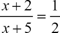. You have one rational expression equal to a constant, so you can cross-multiply. Before doing that, think for a moment about the domain. Because the denominator is x + 5, the domain cannot include − 5. The domain is all real numbers except − 5. Let’s solve.

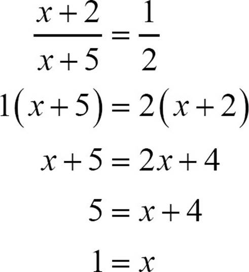
A solution of x = 1 is possible because 1 is in the domain, but you should still check to be sure that it is a valid solution. Check by replacing each x in the equation with 1.

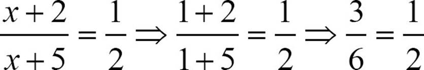
That substitution gives a true statement, so the solution is correct.

Let’s try one that leads to a quadratic equation. Before solving 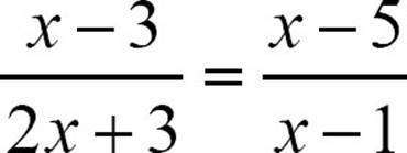, notice that the domain is all real numbers except 1 and . If either of those values turn up as solutions, we’ll reject them as extraneous. Let’s cross-multiply and see where it takes us.

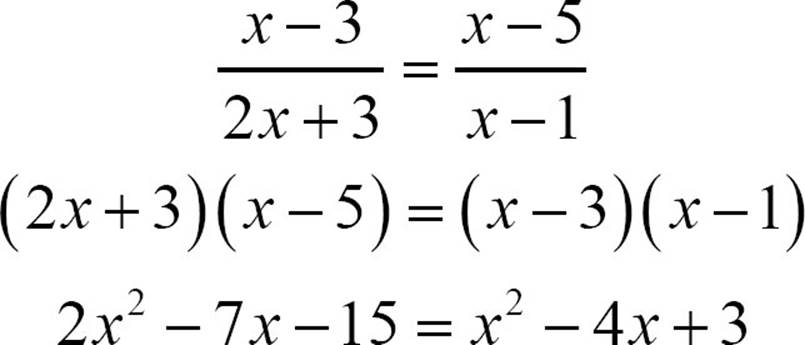
Cross-multiplying is going to leave you with a quadratic equation, so gather up all the terms on one side equal to zero.

x² − 7x − 15 = − 4x + 3

x² − 3x − 15 = 3

x² − 3x − 18 = 0

You can use the quadratic formula if necessary, but it’s worthwhile to try factoring first.

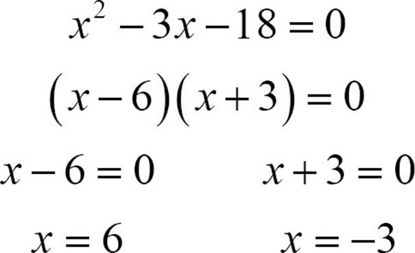
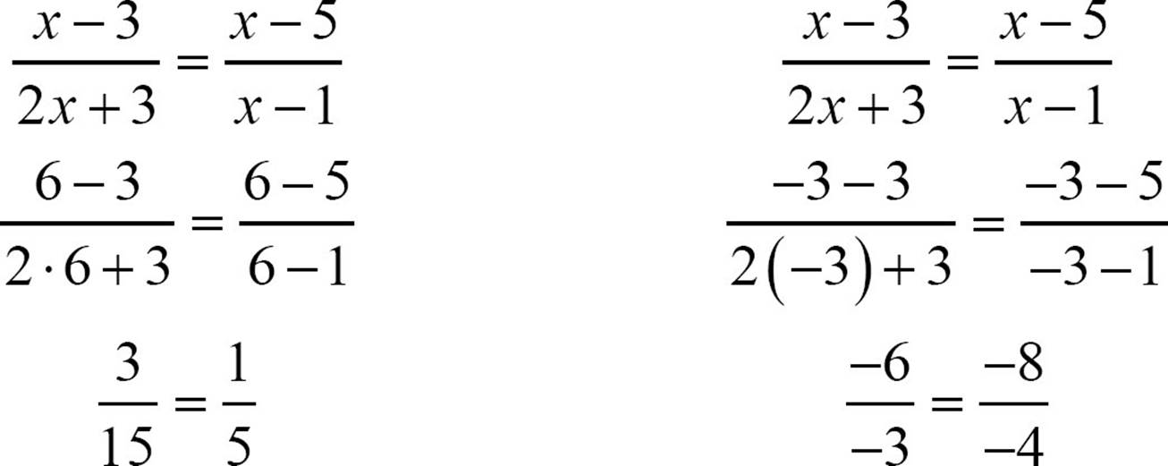
You end up with two solutions. Both are in the domain, but both need to be checked.

ALGEBRA TRAP

Forgetting to check the solutions to a rational equation is one of the most common sources of errors. Extraneous solutions are possible, especially when there are values that are excluded from the domain. Always check rational equations by returning to the original equation so you don’t get confused by any errors in your work.

Both solutions check in the original equation, so the rational equation has two solutions, x = 6 and x = −3.

Cross-multiplying is only possible when you have one rational expression equal to one rational expression (or to a constant), and that may not sound like it covers many rational equations. It doesn’t seem to work for an equation like .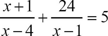

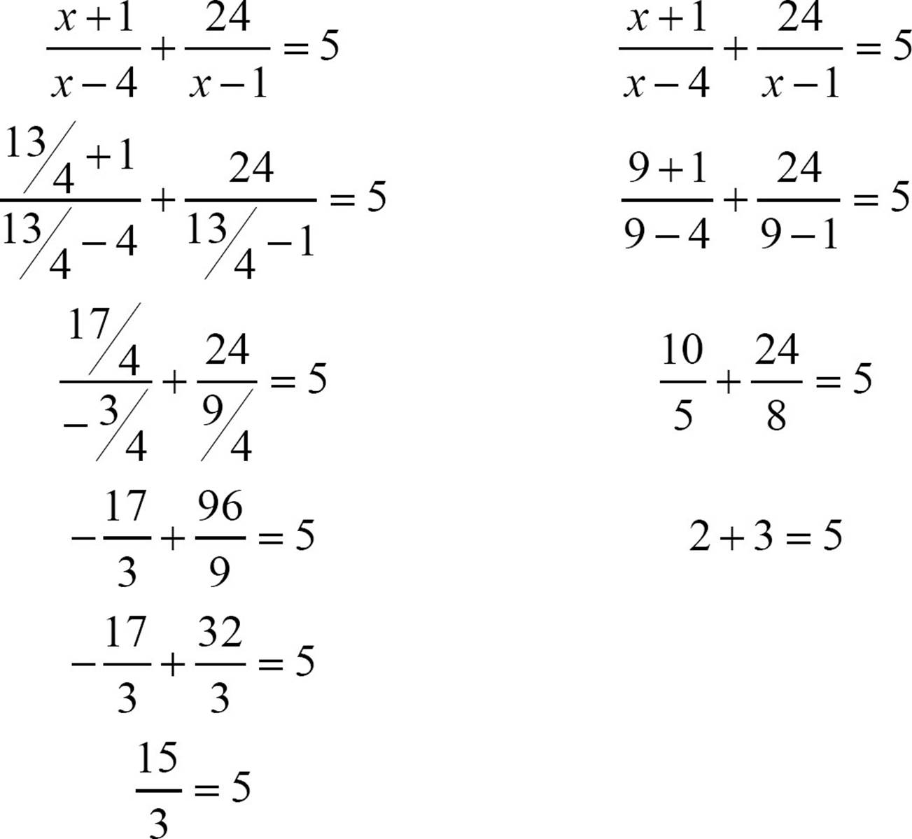
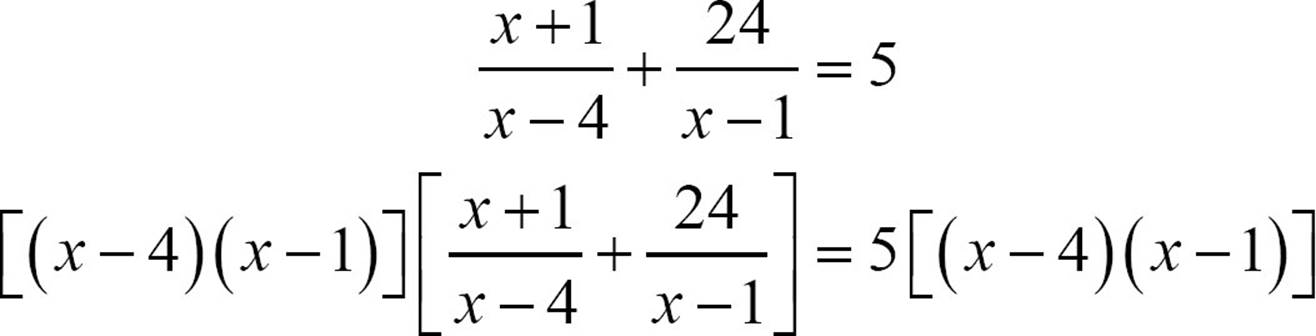
Don’t forget the skills you already have, however. The equation has a sum of rational expressions equal to a constant, but you know how to add rational expressions. You could add those two expressions to create one rational expression that is equal to the constant 5.

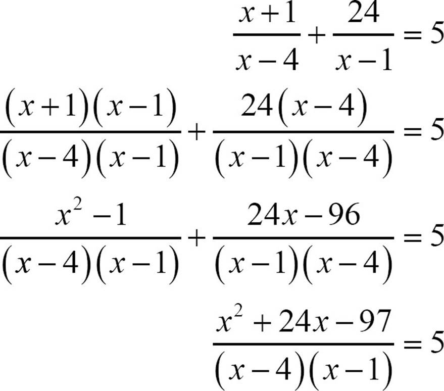
Now you have one rational expression equal to a constant. Multiply out the denominator, put the 5 over 1, and cross-multiply.

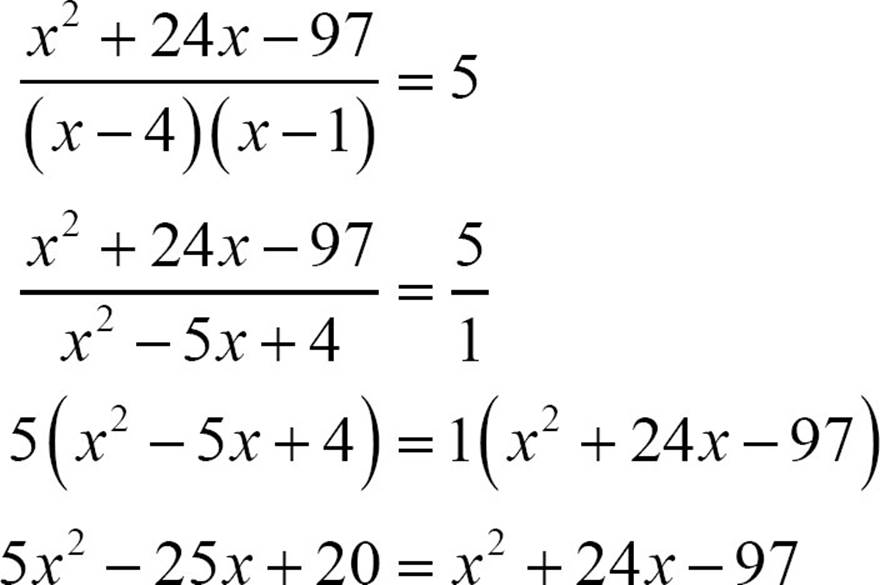
Now you have a quadratic equation, so gather all terms on one side equal to zero.

5x² − 25x + 20 = x² + 24x − 97

4x² − 25x + 20 = 24x − 97

4x² − 49x + 20 = − 97

4x² − 49x + 117 = 0

The size of the coefficients may make you think you need the quadratic formula, and you certainly can use it, but those numbers will be even bigger. It turns out that 117 can be factored as 1·117, 3·39, or 9·13, and that’s not all that many possibilities to try.

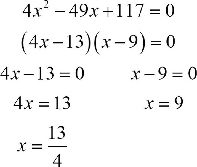
The domain of the equation is all real numbers except 1 and 4, so these solutions are acceptable, but you still should check them back in the original equation.

TIP

When you have fractions inside of fractions you can simplify by multiplying the numerator and denominator of the outer fraction by the denominator of the inner fraction. This will clear the denominators of the inner fractions.

That first check requires patience, but both solutions check. That’s a lot of algebra to solve one equation, even if that equation does have two solutions. Next we’ll look at a technique that may be quicker.

CHECK POINT

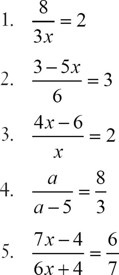
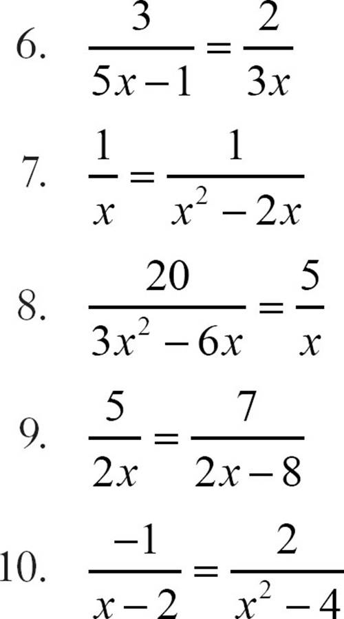
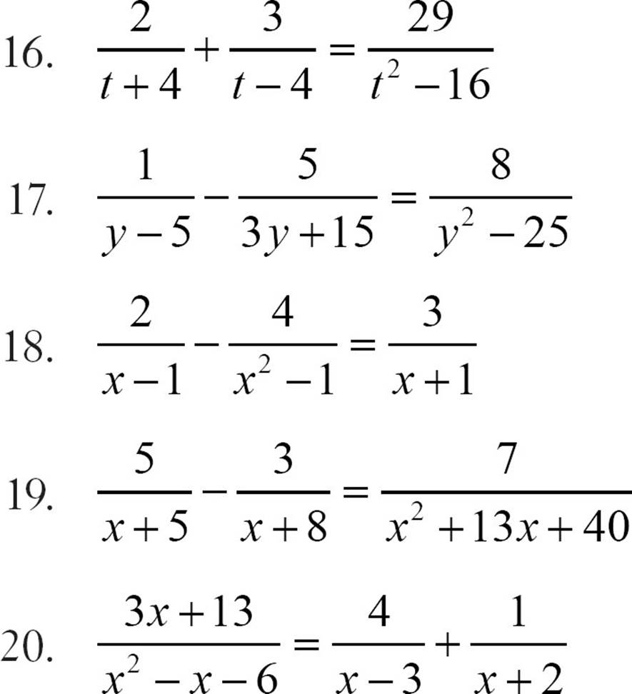
Solve each equation by cross-multiplying. Be sure to check for extraneous solutions.

Multiplying Through

Cross-multiplying is a convenient tactic for solving rational equations that involve only one rational expression, or equations that state two rational expressions are equal. When more operations are involved, however, simplifying the equation enough to use cross-multiplication can be time-consuming. Our second method often proves more practical in those cases.

Let’s revisit 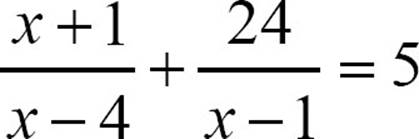, the equation you solved earlier. To use cross-multiplying, you had to add the rational expressions first. Then you cross-multiplied, which resulted in a quadratic equation that you had to solve and check. This time, you’ll use a method called multiplying through to turn the rational equation into a simpler equation quickly. Here’s the plan.

1. Find the common denominator for all the rational equations in the equation.

2. Multiply both sides of the equation by that common denominator, making sure to distribute where necessary. This should eliminate all denominators.

3. Solve the resulting equation.

4. Check any solutions in the original rational equation.

To try this with , you first need the common denominator. The common denominator needs to include a factor of x − 4 and a factor of x − 1, and you don’t need to actually multiply it out. You can leave it in factored form, so the common denominator is (x − 4)(x − 1).

Now multiply both sides of the equation by (x − 4)(x − 1).

It looks rather messy right now, but stay calm and be patient. Distribute on the left side and do some canceling.

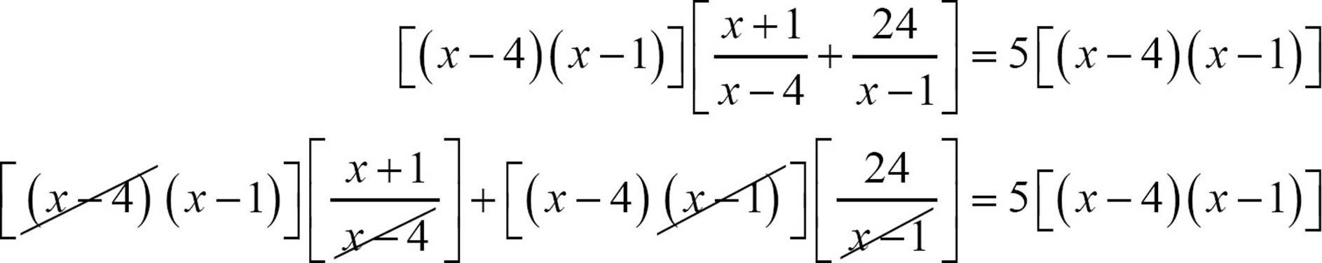
This leaves you with a more manageable equation.

(x − 1)(x + 1) + (x − 4)· 24 = 5 [(x − 4)(x − 1)]

The denominators are gone, so multiply out.

(x − 1) (x + 1) + (x − 4) ·24 = 5 [(x − 4) + (x − 1) ]

(x² − 1) + (24x − 96) = 5 (x² − 5x + 4)

x² + 24x − 97 = 5x² − 25x + 20

You’ve seen this equation before, when you solved it by cross-multiplying, and there’s no need for you to solve it again, but getting to this point was quicker and easier with the multiplying through method.

TIP

If you multiply through and still have a denominator, check to make sure you’ve used the correct common denominator, and that you’ve distributed to every term.

Let’s try another example by multiplying through, and take this one all the way to the end. Suppose you want to solve 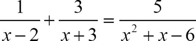. Before looking for the common denominator, factor the last denominator. x² + x − 6 = (x+ 2)(x − 2), so your equation is 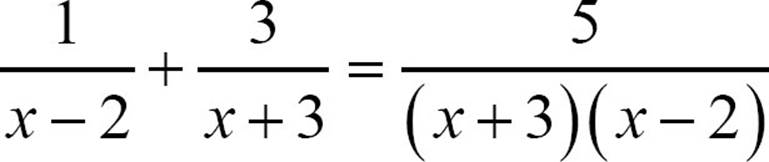, and the common denominator for all three rational expressions is (x + 3)(x − 2).

Multiply both sides of the equation by (x + 3)(x − 2), distributing on the left side.

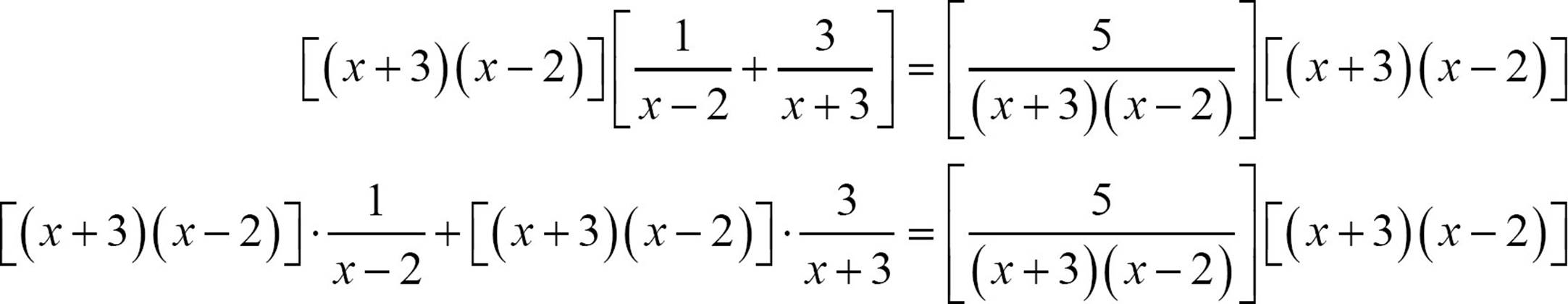
Canceling what you can will eliminate all the denominators.

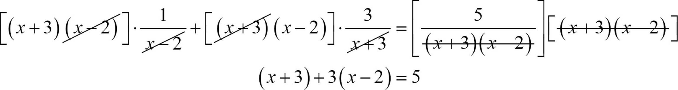
This is a much simpler equation now, so let’s solve. Simplify the left side first.

(x + 3) + 3(x − 2) = 5

x + 3 + 3x − 6 = 5

4x − 3 = 5

4x = 8

x = 2

Don’t forget to check the solution. The values that must be excluded from the domain are 2 and -3, so x = 2 is not an acceptable solution.

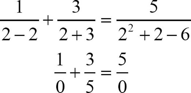
Substituting x = 2 in the original equation will make two of the three denominators equal zero. It cannot be a solution, even though all the algebra was done correctly. x = 2 is an extraneous solution and the equation has no solution.

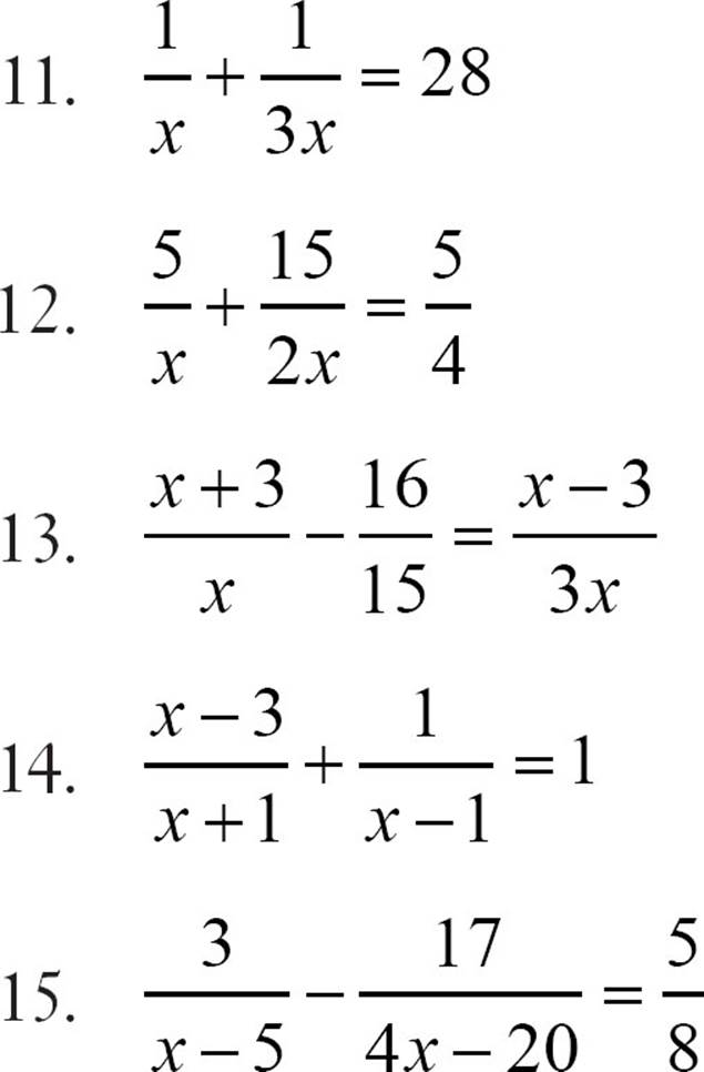
CHECK POINT

Solve each equation by multiplying through. Be sure to check for extraneous solutions.

Graphing Simple Rational Functions

You’ve explored the graphs of several different kinds of functions. Now it’s time to look at the graphs of functions that involve rational expressions, which are quite distinctive.

Because the domain cannot include any values of the variable that will make a denominator equal to zero, the domain of a rational function will usually be limited. Sometimes only one value has to be excluded, sometimes more than one, but even one excluded value will cause a break in the graph. This means that the graph of a rational function is usually in two or more pieces. Rational functions that have more than one value excluded from their domain will have graphs with more pieces. If a rational function is defined for all real numbers, its graph will be one piece.

A rational function for which only one value is excluded from the domain is called a simple rational function. The shape of the graph of a simple rational function is a pair of curves that together are called a hyperbola. They look like a pair of wings turning away from one another.

Let’s begin our look at graphs of rational functions with a simple case, the graph of 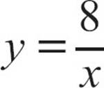. When you graphed parabolas, you learned that to build a good picture of the function, you needed to locate the vertex before setting up our table of values. You found at least the x-coordinate of the vertex so that you could be sure to include a few points to the right and a few points to the left of the vertex.

For rational functions, you want to locate the value that makes the denominator equal to zero. That is the x-value where the function is undefined and therefore where there will be a break in the graph. It’s called a discontinuity. You don’t want to include that value, but you want to make sure that you choose some x-values below the discontinuity and some above it, so that you see both pieces of the graph.

DEFINITION

A discontinuity is the value at which the rational function is undefined, because there is a break in the graph at that value.

For , the value that must be excluded from the domain is x = 0, so we’ll choose some negative values and some positive values for x. We’ll have to calculate the quotient of 8 and our x-value, so we’ll start with factors of 8.

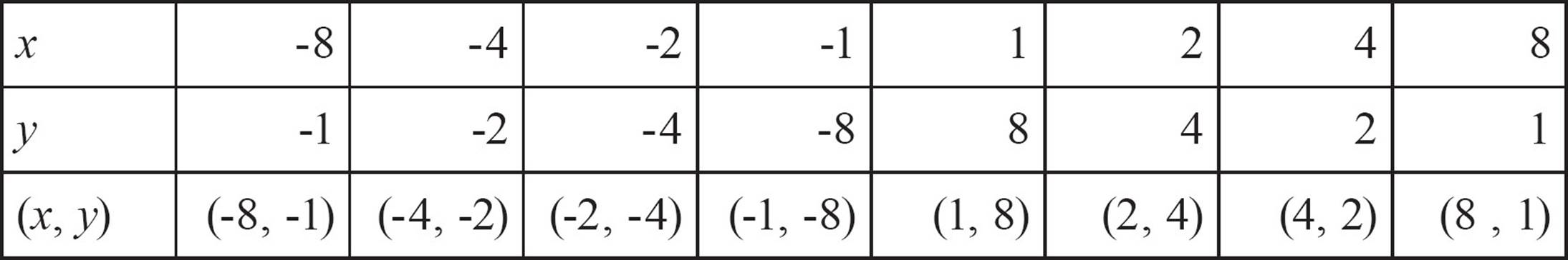
Here’s what it looks like when you plot the points. Can you see the two wings?

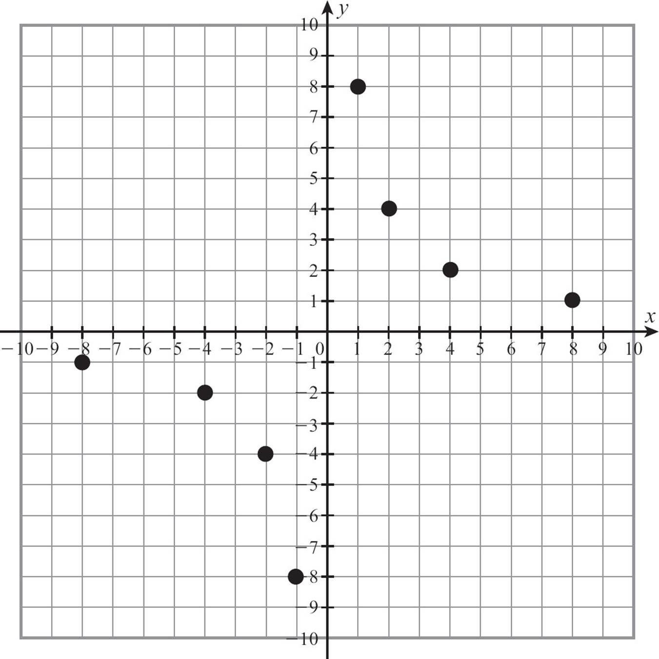
Before trying to connect the dots, there are a couple of key characteristics of the graph to note. You know that there would be a discontinuity, a break in the graph, at x = 0, so it’s important to remember not to try to connect the two segments of the graph. Each wing is a curve, as you may already be able to tell from the points, so put the ruler away. Sketch the curves smoothly. Finally, let’s look at what happens as x becomes very large or very small.

The simplest way to see what happens is to evaluate the function for a few large values of x, and a few small ones.

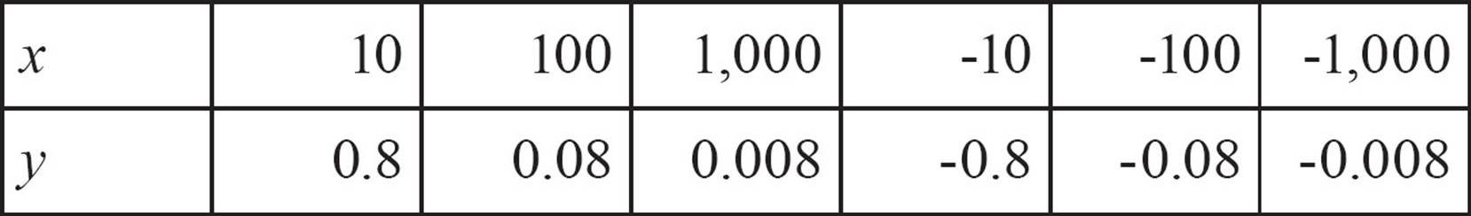
As x becomes very large, the value of y gets smaller and smaller, coming closer to 0, but as long as x is a positive number, will be a positive number. There is no value of x that will ever make y equal zero, so the right wing of the graph will get very close to the x-axis, but will never cross it. In the same way, the left wing will always have negative y-values, getting closer and closer to the x-axis but never touching it.

When you sketch the graph with those concerns in mind, it looks like this.

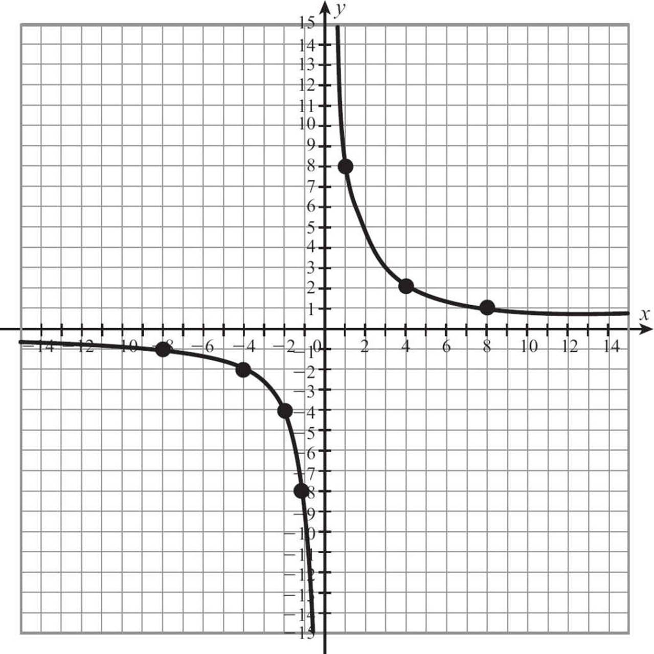
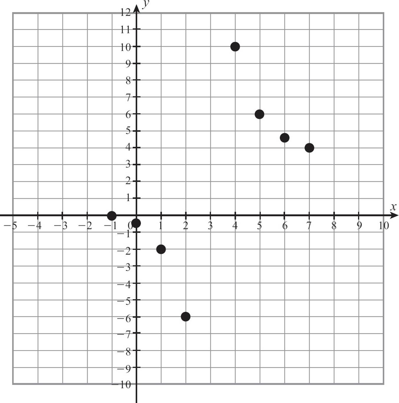
Let’s investigate another example, and this time we’ll make the equation a little more complicated, but just a little. Let’s graph .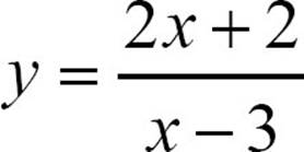

Start by identifying the domain. The denominator is x - 3 so x = 3 would make the denominator zero. The domain is all real numbers except x = 3, and your graph will have a discontinuity at x = 3.

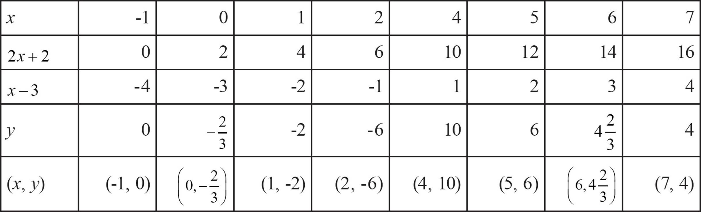
Choose a few values less than 3 and a few greater than 3 to build a table of values.

The shape of the graph is a little harder to spot from these points. The first graph we looked at was compartmentalized by the x-axis and y-axis. Because the graph never crossed those axes, each wing was contained in one quadrant. Here the boundaries aren’t as clear, but if you stop to think for a moment, you can find them.

You know that x = 3 is not in the domain, so there will be a discontinuity there. Draw in the vertical line x = 3 as a dotted line on the graph.

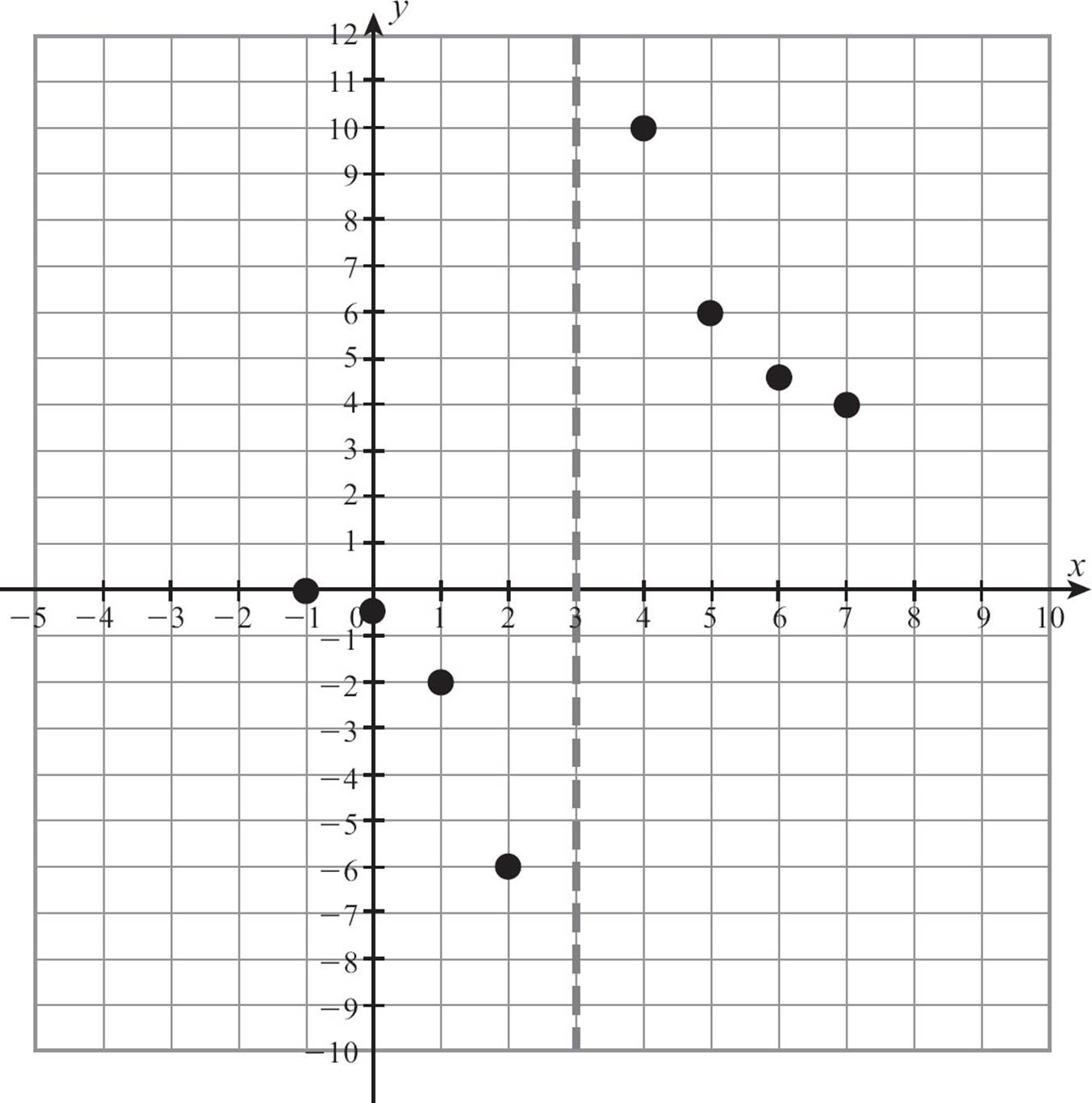
That divides the two wings, the way the y-axis did in our first example. That first example also had the x-axis as a dividing line between the two wings, with both getting close to the x-axis but never touching it. That’s not the case here. You already have a point on the x-axis. Let me show you a few more points that fit our equation. I think you’ll be able to guess where the dividing line is.

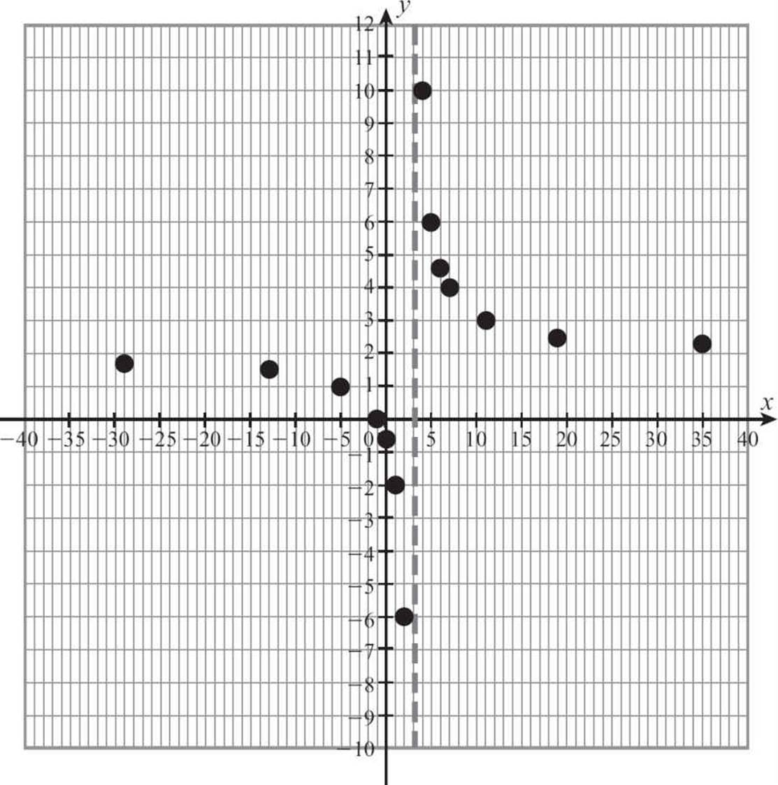
Can you see that y = 2 is the dividing line? If you add a dotted line there, and sketch in the graph, it looks like this.

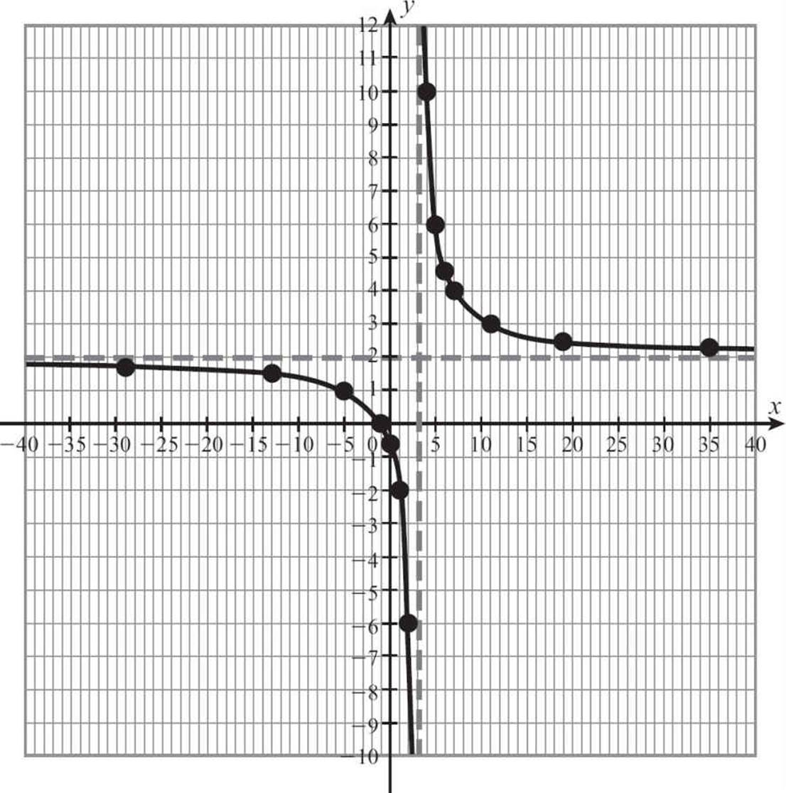
Asymptotes

Those two dividing lines, the vertical line and the horizontal lines that the graph gets very close to but doesn’t touch, are called asymptotes. Although they’re not part of the graph, knowing where they are helps us draw the graph of the rational function. Because the asymptotes are helpful, having a quick way to find them would make the task of graphing a rational function easier.

DEFINITION

An asymptote is a line that a graph approaches very closely. The graph never crosses a vertical asymptote.

The vertical asymptote is easy to locate, and in fact, you find it every time you start to graph a radical function. The first thing you do is find the value that must be excluded from the domain, the location of the discontinuity, and that’s where the vertical asymptote is. If you find that x = −4 makes your denominator zero, then x cannot equal −4, so there’s a break in the graph there. The discontinuity occurs at −4, and the equation of the vertical asymptote is x= −4.

The horizontal asymptote takes a little more work, but for simple rational functions, you can find it with one of two rules.

1. If the degree of the numerator and the degree of the denominator are the same, as they are in 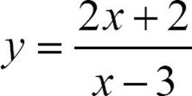, divide the highest power term of the numerator by the highest power term of the denominator. In our example , so our horizontal asymptote is y = 2.

2. If the degree of the numerator is less than the degree of the denominator, as it is in , the horizontal asymptote is y = 0, the x-axis.

You might be wondering if there’s a third rule for when the degree of the numerator is higher than the degree of the denominator. You could call it a rule, I guess, but if that happens, there’s no horizontal asymptote. That won’t occur in simple rational equations.

Intercepts

As you saw when you graphed , not every rational function will have an x-intercept or a y-intercept, but when there are intercepts, they’re easy to find and helpful for graphing. By replacing x with 0 and simplifying, you can find the y-intercept. When there is no y-intercept, you’ll have an expression like , which is undefined.

To find the x-intercepts, replace y with 0 and solve the equation. For a simple rational function like , doing that will give you an equation you’ll want to solve by cross-multiplying.

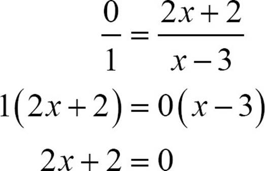
Solving a simple rational function to find the x-intercepts turns into finding the values of x that make the numerator equal zero.

THINK ABOUT IT

Replacing y with 0 and solving the resulting rational equation will turn into solving for values that make the numerator zero. For a rational expression, a fraction, to equal zero, the fraction must be zero over a non-zero number. No other quotient can equal zero.

Step-by-step, here’s the plan for graphing simple rational functions.

1. Find the value of x that will make the denominator equal zero. This value is not in the domain, but it is the location of the vertical asymptote. Draw a dotted vertical line for the vertical asymptote.

2. Find the horizontal asymptote by following our two rules (y = 0 or 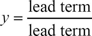). Draw a dotted horizontal line for the horizontal asymptote.

3. The two asymptotes divide the plane into four sections. The two wings of the hyperbola will be in two of the four.

4. Find the y-intercept if there is one, by substituting 0 for x and simplifying. Plot the y-intercept.

5. Find the x-intercept, if there is one, by finding the values of x that make the numerator equal to zero. Plot the x-intercept.

6. Make a table of values, using as many values as necessary to define the curves. Be sure to choose values on both sides of the vertical asymptote.

7. Draw each wing by connecting the points with a smooth curve. Do not connect the two wings. Do not cross the asymptotes.

TIP

For simple rational functions in which x-terms are first degree, the two wings will be in diagonally opposite sections. The wings will be either in the upper right and lower left sections, or in the lower right and upper left. But when higher powers of x are involved, you may find the wings in side-by-side sections.

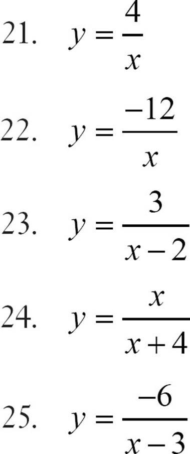
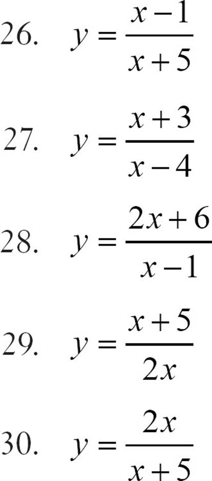
CHECK POINT

Graph each rational function by finding asymptotes and intercepts, and making a table of values if necessary.

The Least You Need to Know

·  Solve rational equations that are two equal rational expressions by cross-multiplying. Solve the resulting equation and be sure to check your solution.

·  Solve multi-term rational equations by multiplying through by the common denominator of all rational expressions involved. Solve the resulting equation and check your solution.

·  Simple rational functions have a graph called a hyperbola.

·  The vertical asymptote(s) occurs at the point(s) of discontinuity. The horizontal asymptote occurs at the ratio of the lead terms, or at the x-axis.

·  Sketch the graph of the rational function by finding the vertical and horizontal asymptotes, the intercepts if any, and then building a table.