Idiot's Guides: Algebra I (2015)
Part II. Linear Relationships
Chapter 6. Graphing Linear Functions
In This Chapter
![]()
· Understanding the coordinate plane
· Graphing using a table of values
· Quick graphing by intercept-intercept or slope-intercept
· Understanding direct variation relationships
A picture is worth a thousand words, according to the old saying, and pictures can be just as valuable in helping us understand equations and functions. The pictures that represent equations and functions tend to be one picture for one equation rather than one picture for a thousand of anything, but these pictures, or graphs, make patterns clearer.
We’ve already talked a little bit about graphs when we first looked at functions, and we saw that the graph gave us a quick way to tell if a relation was a function. In this chapter, we’ll focus on the graphs of an important group of functions, called the linear functions. We’ll see why they have that name, and we’ll look at quick graphing methods and one important application.
The Cartesian Plane
The system of graphing that you’re probably accustomed to using is a rectangular coordinate system, or coordinate plane. It gets its formal name, the Cartesian coordinate system, from Rene Descartes, a seventeenth-century French mathematician and philosopher. Using this system, you locate each point by a pair of numbers, called an ordered pair because the order of the numbers is important. The first number tells you how many spaces to move left or right, and the second number indicates movement up and down.
![]()
DEFINITION
The Cartesian plane, or coordinate plane, is a system of identifying every point in the plane by an ordered pair of numbers. The plane is divided into four sections, called quadrants, by a horizontal line, called the x-axis and a vertical line called the y-axis, which intersect at the point called the origin. The first number in the ordered pair tells how to move left or right from the origin and the second number tells how to move up or down.
All this movement starts from a point called the origin, which is the intersection of a horizontal line and a vertical line. The horizontal line is generally called the x-axis and the vertical line is the y-axis. The origin is the point (0, 0). On the x-axis, positive numbers go to the right and the negatives to the left, just like a number line. On the y-axis, positives go up and negatives down.
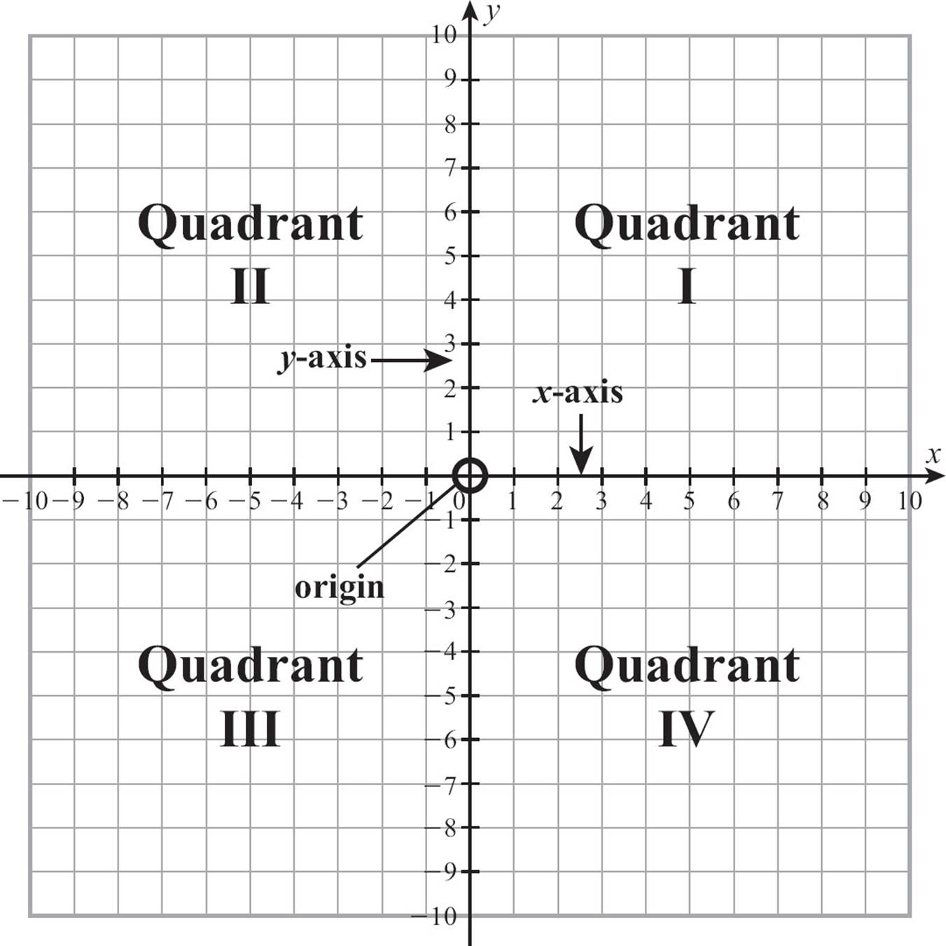
The x-axis and y-axis intersect at the origin and divide the plane into four sections called quadrants. The quadrants are referred to by numbers, starting from the upper right and going counterclockwise.
![]()
THINK ABOUT IT
The graphing we’re talking about draws pictures on a flat surface, or plane. You can think of a plane as a piece of paper that never ends, but it’s basically two-dimensional, which is why two coordinates are all you need to locate a point. If you were working in three dimensions, you’d need three axes, and three coordinates. The third number would tell you to move up above the page or down below it.
![]()
CHECK POINT
Plot each point on the Cartesian plane.
1. (-4, 7)
2. (6, -2)
3. (0, 4)
4. (-3, -1)
5. (-2, 0)
Use the figure to answer questions 6 through 10.
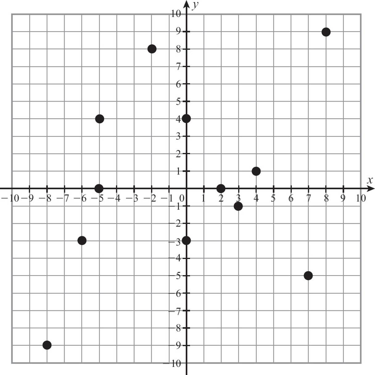
6. Give the coordinates of a point in the first quadrant.
7. Give the coordinates of a point on the y-axis.
8. Give the coordinates of a point in Quadrant IV.
9. Give the coordinates of a point in Quadrant III.
10. Give the coordinates of a point on the x-axis.
Graphing Linear Functions
In an earlier chapter on functions, we talked about graphing pairs of numbers as points in the plane to help decide if a relation is a function, and if it follows a pattern. One of the most common patterns you will see is a line. Functions whose graphs form a line are called linear functions. The pattern can be represented by an equation, which can be written using function notation. Throughout this chapter, we’ll use “linear function” and “linear equation” interchangeably.
![]()
DEFINITION
A linear function is a function of the form y = mx + b. It defines the value of the output variable as a multiple of the input variable, possibly plus or minus a constant.
You can recognize a linear function by looking at its rule. The rule has a term that includes the input or independent variable, raised to the first power. You won’t see any exponents or roots. If there’s a fraction, the denominator contains only numbers, never variables. There may or may not also be a constant term. f (x) = − 7x is a linear function, and so is 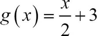 , but
, but 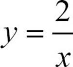 and p (x) = x2 − 4x + 6 are not linear functions.
Table of Values
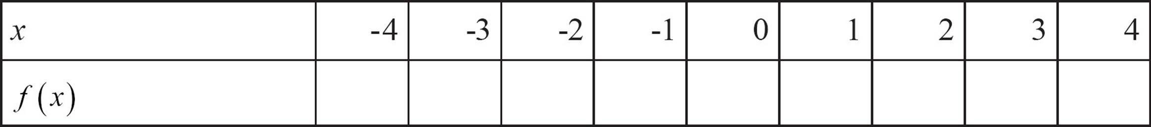
The most basic way to graph a linear function—or any function, for that matter—is to use the rule to build a table of values. If the rule for your function is f (x) = 2x − 5, you can choose several values for the independent variable, x, to build a table. It’s wise to choose both positive and negative values for x. You’re not saying these values are the entire domain of the function. You’re just using them to give an idea of what the graph looks like.
Putting the values you’ve chosen in order makes them easier to plot, but there’s no rule that says you have to choose consecutive numbers for your table. If there are fractions involved in the rule you’re going to evaluate, you can choose numbers that are divisible by the denominator. If you need to multiply your inputs by ![]() , for example, you can choose to use only multiples of three to eliminate fractions.
, for example, you can choose to use only multiples of three to eliminate fractions.
Once you’ve chosen the values for the independent variable, you evaluate 2x − 5 for each value.
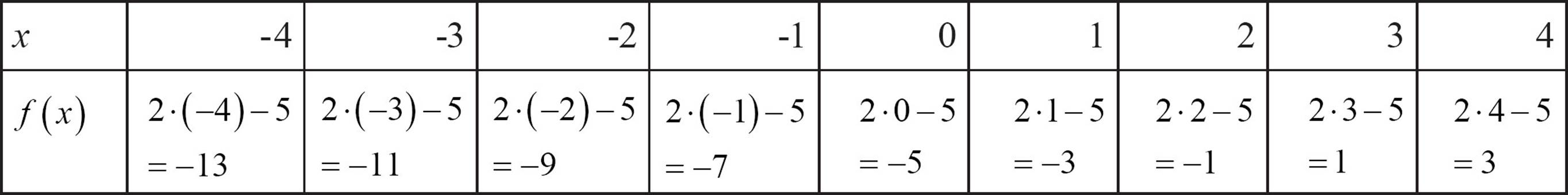
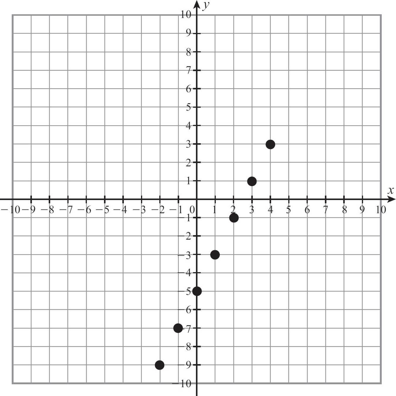
The table of values now gives you a set of points that belong to the function. It’s not the whole function. You’re assuming the function has a domain of all real numbers. These points should be enough to show you the pattern, however, so plotting them will be the next step.
![]()
DEFINITION
The domain of a function is the set of all values that can be substituted for x, all possible inputs. The range is the set of all outputs, all values of y.
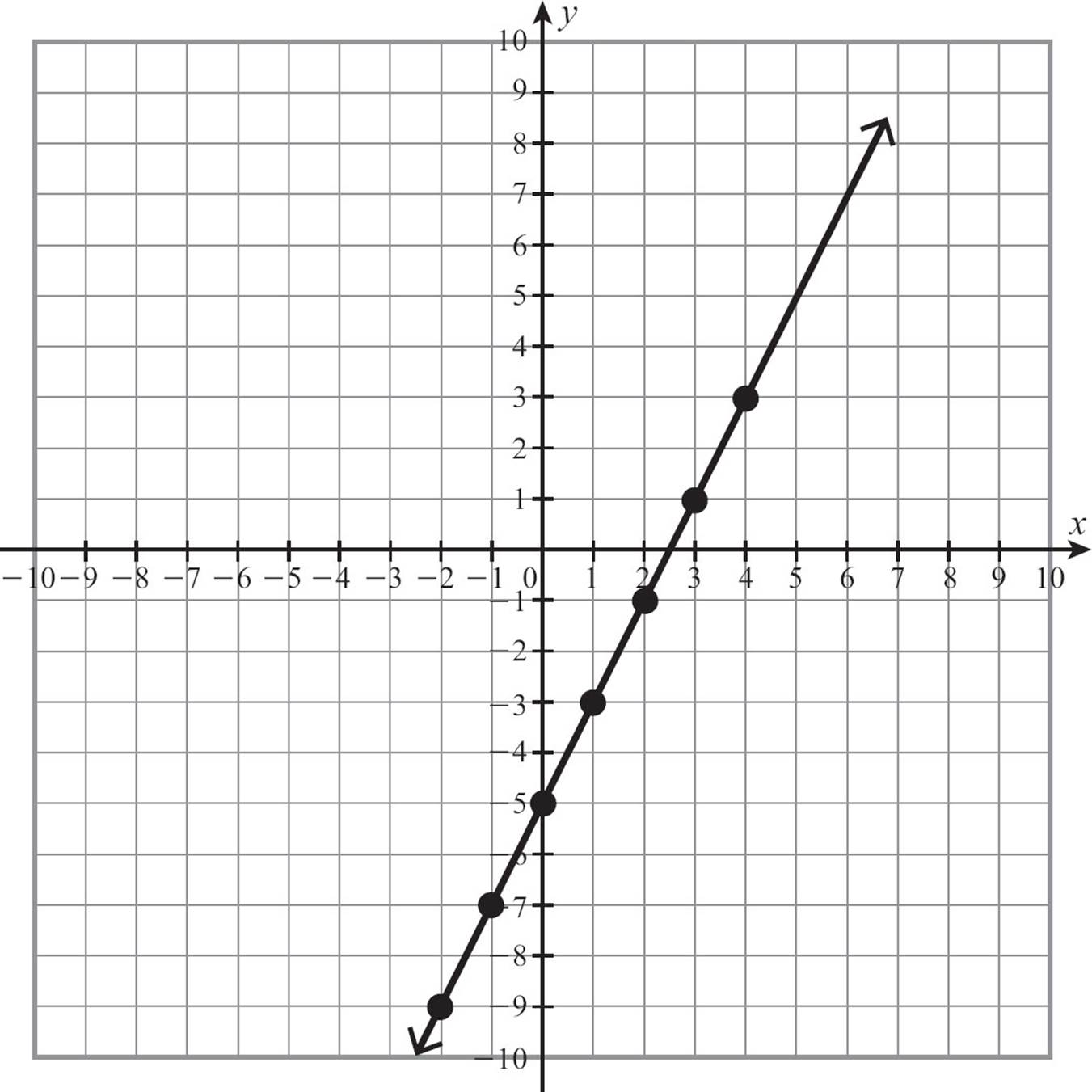
Once the pattern is clear, you just need a straightedge to draw the line. Add arrowheads on the ends of the line to communicate the fact that it continues beyond what you’ve drawn.
![]()
CHECK POINT
Graph each function by making a table of values and plotting points.
11. f (x) = 3x − 4
12. 
13. y = 2x − 3
14. g (x) = x + 5
15. y = − x + 5
16. f (x) = −2x + 7
17. 
18. y = 4 − 3 x
19. f(x)= − 2x
20. 
After building a few tables of values, you may have begun to notice some patterns, or perhaps patterns in the patterns. Those are going to lead to some shortcuts for graphing linear functions without having to build the whole table of values. You probably noticed that whenever you chose zero as a value of x, the arithmetic was easy. That’s at the heart of the first shortcut.
Intercepts
The x-axis and y-axis are the backbone of the coordinate system. The point at which a graph crosses an axis is called an intercept. The graph crosses the x-axis at the x-intercept, and crosses the y-axis at the y-intercept. Intercepts may not seem especially important. They are just points of the graph that happen to sit on an axis. But geometry dictates that two points are enough to define a line, and every point on an axis has a particular trait in common: one of its coordinates is 0. The x-intercept of a graph is a point that has a y-coordinate of 0. The y-intercept of a graph is a point that has an x-coordinate of 0. Zeros make for easy arithmetic, and quickly give you two points to define the line.
![]()
ALGEBRA TRAP
The intercept-intercept method won’t work if the y-intercept is 0, because the x-intercept will also be 0. Both intercepts are at the origin, so you only get one point instead of two. You can’t tell where the line goes with only one point. You’ll need to use a different method.
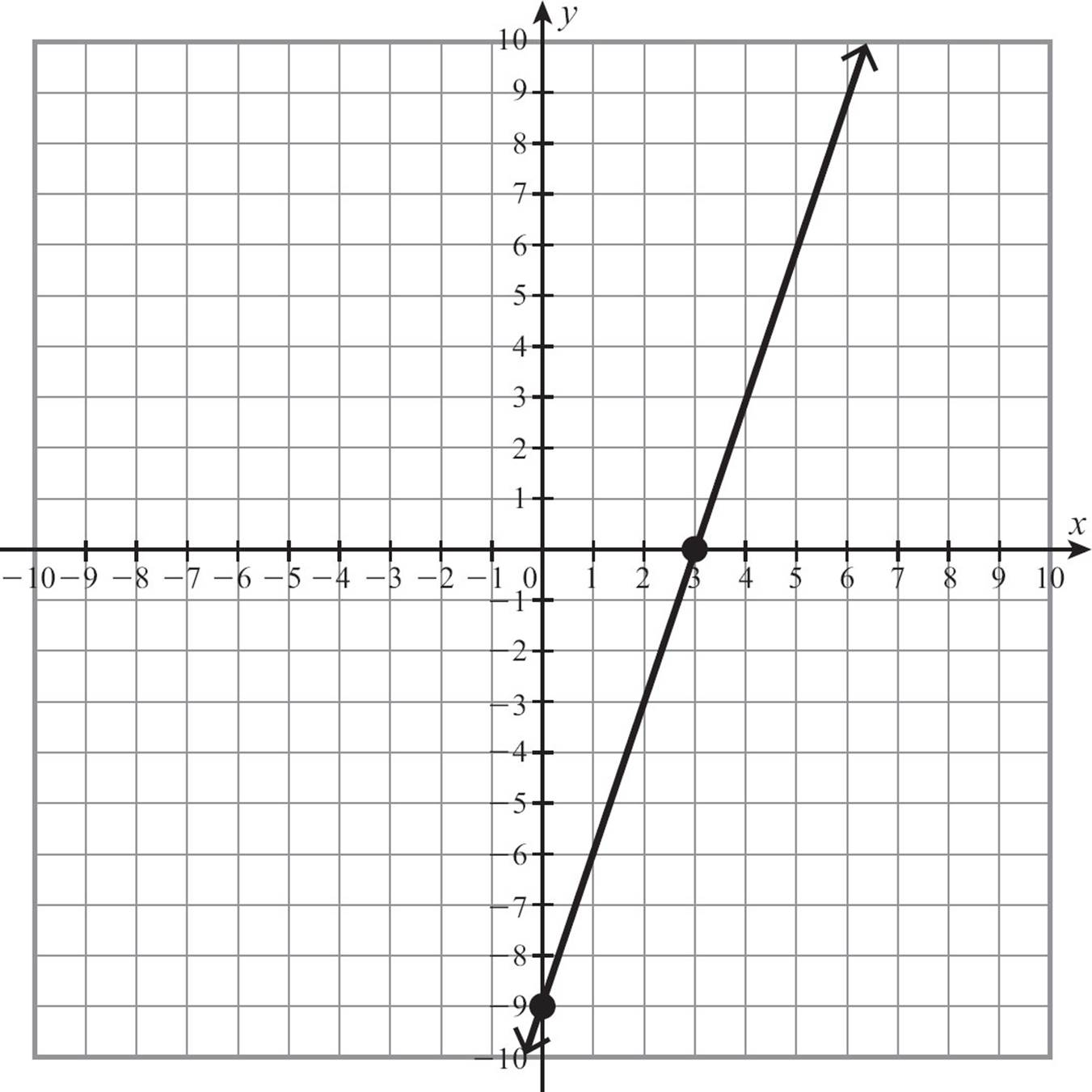
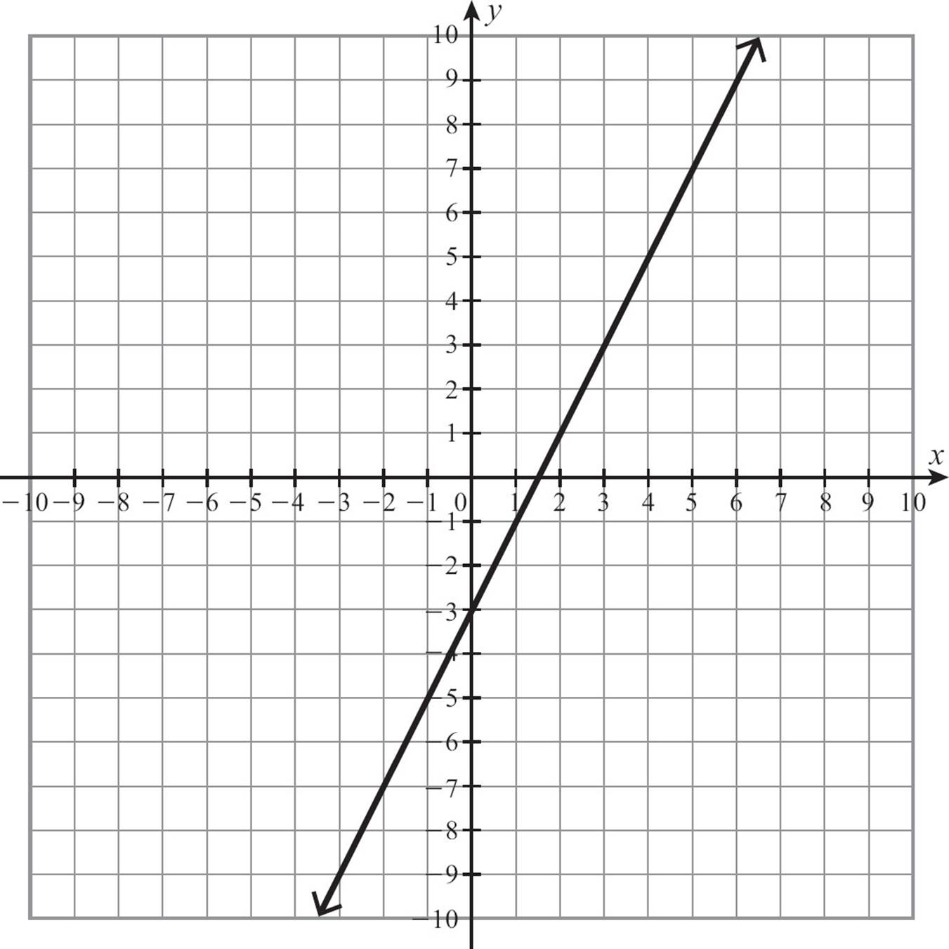
To graph a linear function like f (x) = 3x − 9, begin by writing it as y = 3x − 9. Find the y-intercept by replacing x with 0. y = 3 · 0 − 9 = − 9. The y-intercept is (0, –9). Then find the x-intercept by replacing y with 0. This may require a little bit of algebra, but it shouldn’t be too tough.
0 = 3x − 9
9 = 3x
3 = x
The x-intercept is (3, 0). If you plot (0, –9) and (3, 0), you can use a straightedge to connect them into a line.
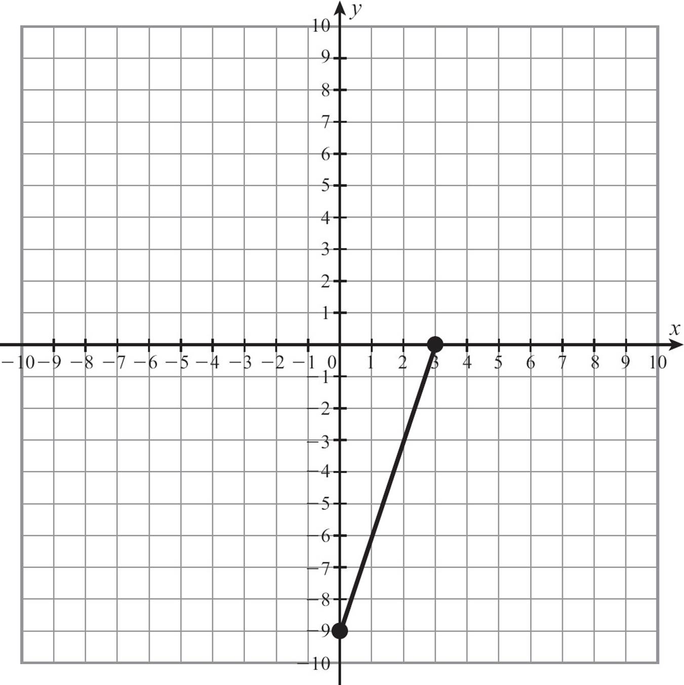
Extend the line and add arrowheads on the ends, and you have the graph of y = 3x − 9.
![]()
CHECK POINT
Find the x-intercept and y-intercept of each function.
21. y = 2x − 6
22. y = −3x + 6
23. y = 4x + 4
24. y = 5 − x
25. y = x + 4
Graph each function using intercepts.
26. y = − 2x + 8
27. y = 3x − 6
28. y = x − 6
29. y = x + 5
30. 
When you built tables of values, you noticed that letting x equal 0 left you with easy arithmetic. That led to the intercept-intercept shortcut. When you were working with intercepts, did you notice there was a way to spot the y-intercept quickly? That ability to spot a y-intercept quickly is going to take you to another shortcut.
Slope and y-intercept
As you worked with the intercept-intercept method, you may have noticed that if the equation of the linear function was in the form y = variable term + constant, that constant term was always the y-intercept. You needed to do some math to find the x-intercept, but the y-intercept was just sitting there.
![]()
TIP
If you don’t see a constant term, the y-intercept is 0 and the line passes through the origin.
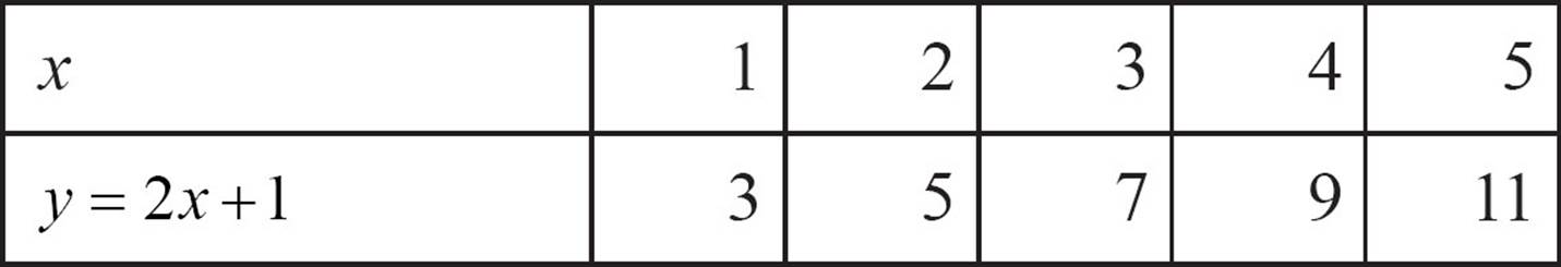
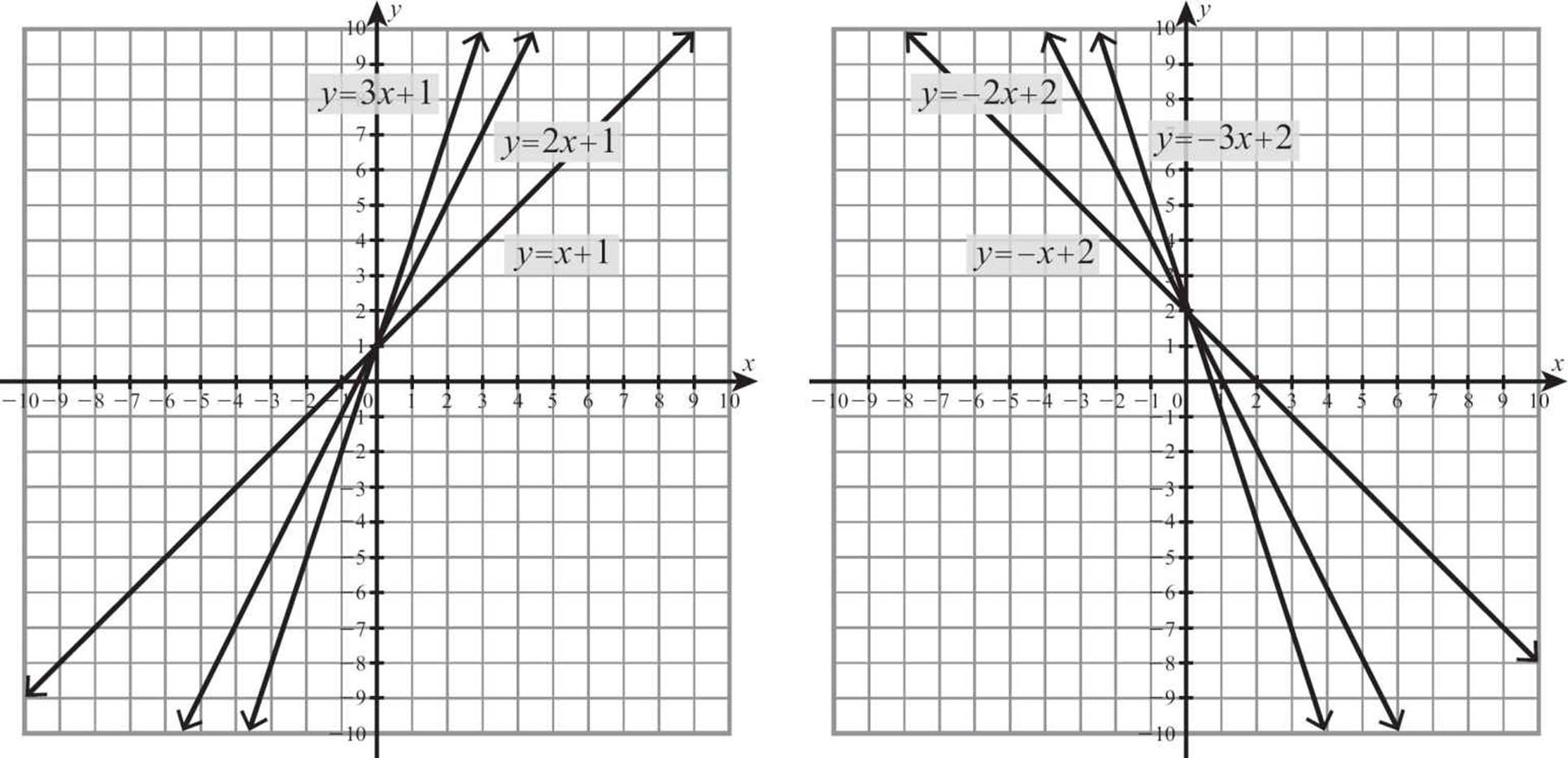
You might have noticed something else surprising when you made tables of values. If you picked inputs in sequence, the change in the output as you went from one to the next was equal to the coefficient of the variable term. If you made a table for y = 2x + 1 and chose your x values that were consecutive, like 1, 2, 3, 4, and 5, the y values went up by twos.
If you change the function rule to y = 3x + 1, the increase in y at each step will be 3.
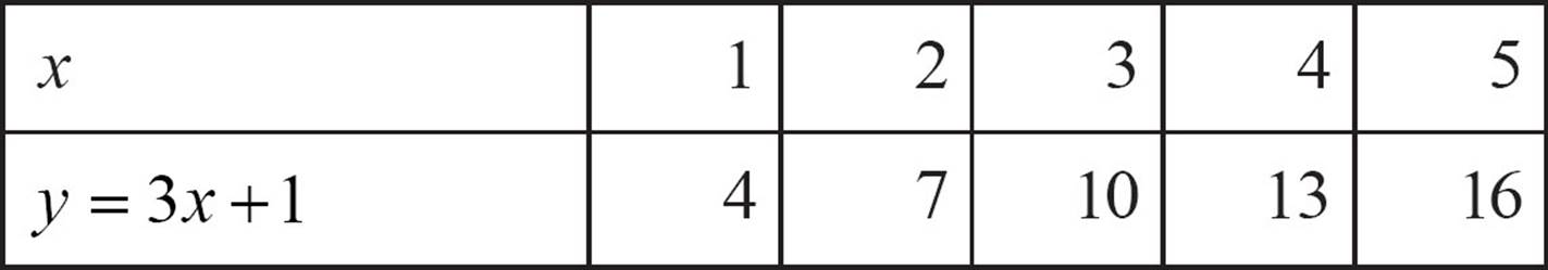
That constant rate of change you’re noticing is called the slope of the line. If the coefficient of the variable term is positive, the line will rise from left to right. If the coefficient is negative, the line will fall. A horizontal line, which neither rises nor falls, has a slope of zero. The larger the absolute value of the slope, the steeper the rise or fall of the line.
![]()
DEFINITION
The slope of the graph of a linear equation is the coefficient of the x-term, and tells how much the line rises or falls each time you move one unit right.
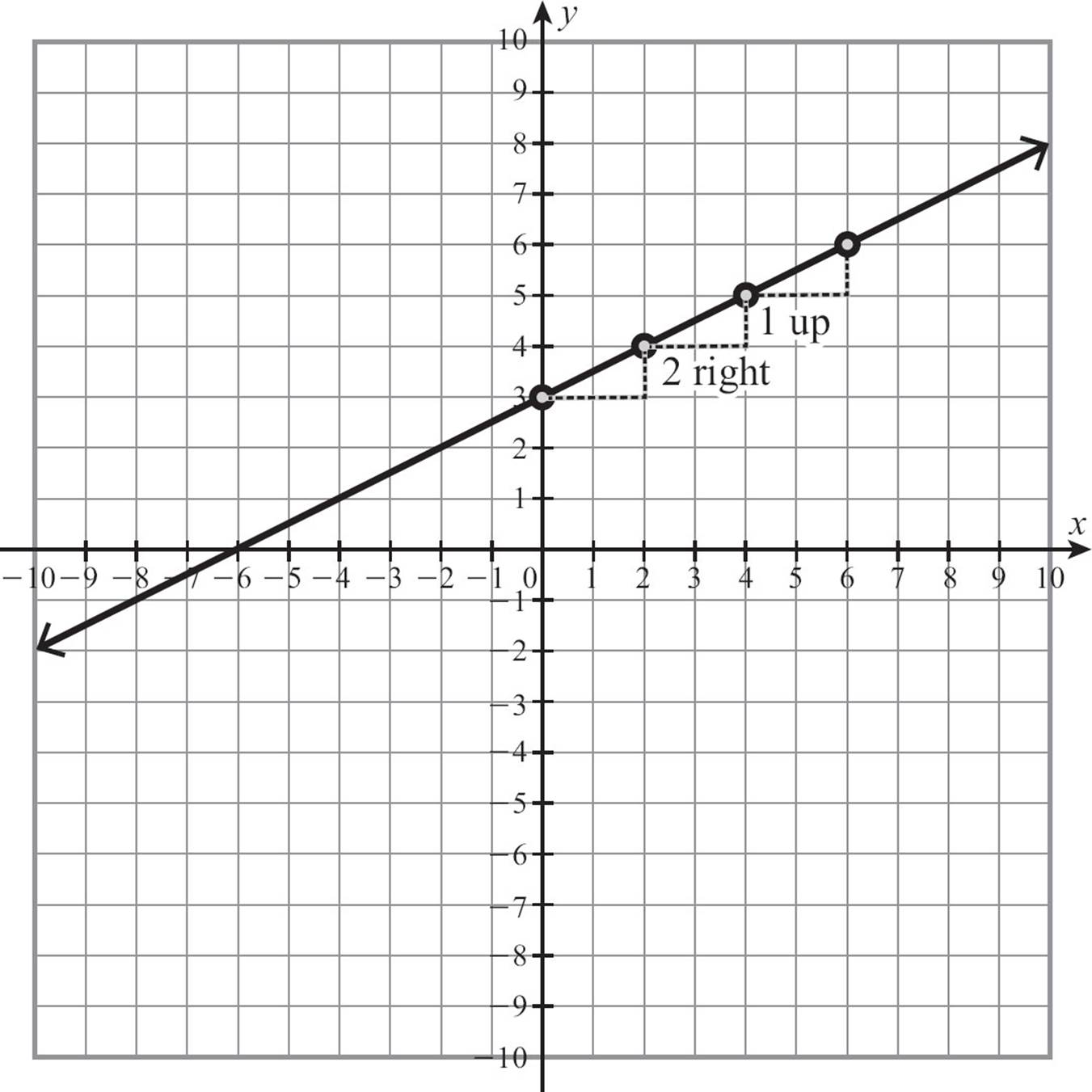
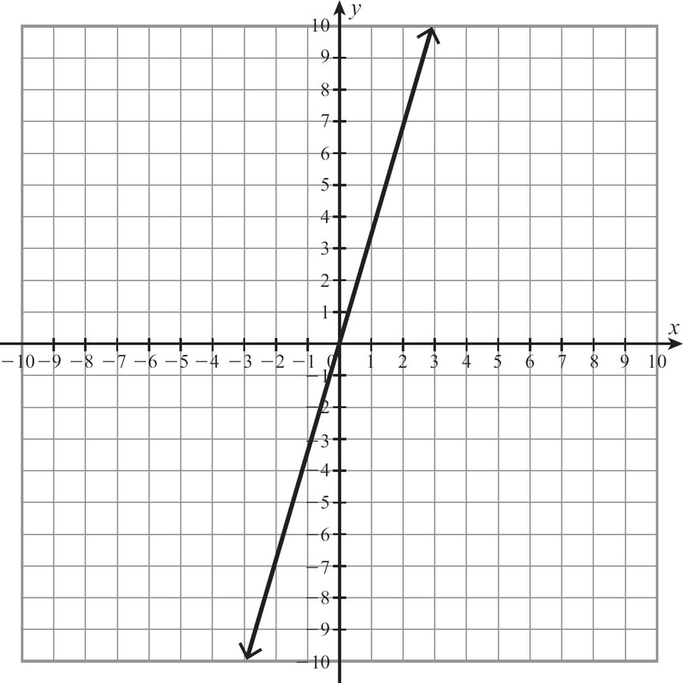
Once you understand what these two numbers, the slope and the y-intercept, tell you about the graph of the function, you can use them to draw the graph quickly. To graph  , first identify the y-intercept. In this equation, that’s the constant term, 3, or (0, 3). Plot the point (0, 3) on the y-axis.
Next, focus on the slope, in this case, ![]() . That tells you that each time you increase the x-coordinate by 1, you increase the y-coordinate by
. That tells you that each time you increase the x-coordinate by 1, you increase the y-coordinate by ![]() . Because most graph paper isn’t marked in half boxes, this could be tricky, so instead of counting over 1 and up
. Because most graph paper isn’t marked in half boxes, this could be tricky, so instead of counting over 1 and up ![]() , count over 2 and up 1. That’s still equivalent to
, count over 2 and up 1. That’s still equivalent to ![]() , but gives you a convenient way to think about the slope. The denominator tells you how much to move over, and the numerator tells how much to move up or down. This is why we talk about the slope as the ratio
, but gives you a convenient way to think about the slope. The denominator tells you how much to move over, and the numerator tells how much to move up or down. This is why we talk about the slope as the ratio  .
.
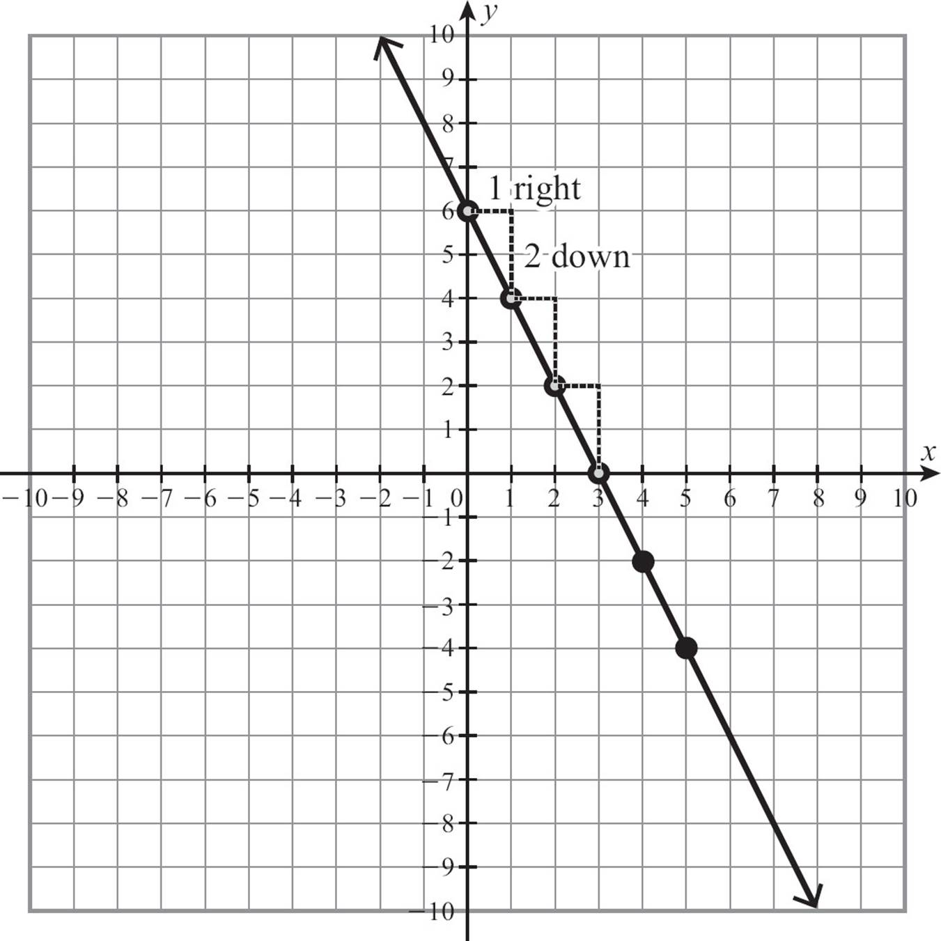
Starting from the y-intercept, count 2 units to the right and up 1. Plot a point. Do it again. From where you just placed the point, count 2 units right and 1 up and plot a point. After you’ve done that a few times, you’ll be able to connect the points into a line.
If the slope of the linear function is a negative number, count right and down. For the line y = −2x + 6, start at the y-intercept (0, 6), make the slope of -2 a fraction by writing it as  , and then count over 1 and down 2, over 1 and down 2. Connect the dots in a line.
![]()
ALGEBRA TRAP
If the slope is negative, be careful. You can count it as  , down is a negative direction, and right is a positive direction. A negative over a positive gives you a negative slope. If you must, you can count it as
  , a positive direction over a negative direction. But don’t get carried away. If you go left and down, you’ll have a negative over a negative and wind up with a positive slope.
We say that 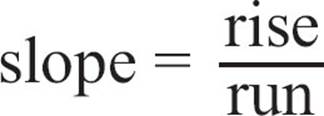 but when the slope is negative, that’s really
  if you’re moving from left to right. Count the run moving to the right, and let the sign of the slope tell you whether to rise or fall.
The combination of the y-intercept and the slope, both of which are easily identified just by looking at the equation, allows you to draw the graph quickly by following these steps.
1. Identify the y-intercept and plot that point.
2. Identify the slope. If the slope is a whole number, make it a fraction by giving it a denominator of 1.
3. From the y-intercept, count up or down the number in the numerator of the slope and over to the right the number in the denominator. Place a dot.
4. Repeat several times. Connect the dots into a line.
![]()
TIP
Sometimes when you’re graphing, you may find that you just can’t count the slope from right to left, usually because going in that direction will run off the page. You have to go “backward” or to the left. That reverses your run, so you need to reverse your rise or fall as well.
![]()
CHECK POINT
Graph each function by slope and y-intercept.
31. y = 2x − 5
32. y = 3x − 7
33. y = −4x + 9
34. 
35. 
36. 
37. y = −x + 5
38. y = 2x − 9
39. y = 2x + 3
40. y = −2x + 1
There are a great many situations that can be modeled by linear functions, but one in particular is very common and happily, very simple.
Direct Variation
When two quantities are related and one changes, the other changes as well. If you buy two doughnuts, you might pay $1.78. If you decide you’re hungry and add a third doughnut to your order, the price will increase to $2.67. The price varies with the number of doughnuts you buy.
There are different kinds of variation, but the most common one, direct variation, is modeled by a simple linear equation. When two quantities vary directly, one is a constant multiple of the other. If muffins are $2 each, the price of an order of muffins is $2 times the number of muffins. The cost, C, of the order varies directly with the number of muffins, m, and you can describe that with the equation C = 2m. Direct variation relationships always fit that simple equation. There is no (non-zero) constant term, and nothing going on except one variable being multiplied by a constant to produce the other.
The constant multiplier is called the constant of variation, and it is usually denoted as k. The general pattern of a direct variation equation is y = k x. The specific equation of a direct variation relationship has that form, but uses the particular variables from the relationship and fills in the value of k. C = 2m is the particular equation of our muffin example. That’s a linear function with a slope of 2 and a y-intercept of 0. In any direct variation relationship, the equation is a linear equation with a slope of k and a y-intercept of 0.
![]()
THINK ABOUT IT
If y varies directly with x, it’s also true that x varies directly with y. If y = 2 x,  . Both are direct variation, but the constant of variation is different.
Do you remember that doughnut example? If you buy 2 doughnuts, you pay $1.78, but if you buy 3, you pay $2.67. It’s a direct variation relationship, but what’s k? Let’s say n is the number of doughnuts and P is the price. P varies directly with n, so P = kn. You don’t know the value of k, but you can find it. Plug in what you do know: when n = 2, P = 1.78 or when n = 3, P = 2.67, P = kn becomes 1.78 = k · 2 and dividing both sides by 2 tells you that  . The particular equation for the doughnut example is P = 0.89n. You could use that equation to figure out that 6 doughnuts would cost P = 0.89 · 6 = $5.34.
![]()
CHECK POINT
In questions 41 through 45, tell whether the relationship is a direct variation relationship.
41. y = 3x
42. y = 5x − 3
43. xy = 12
44. 
45. 
46. Distance traveled, d, and time spent traveling, t, vary directly. If you travel 90 miles in 2 hours, what is the constant of variation?
47. The circumference, C, of a circle varies directly with its radius, r. If C = 20π when r = 10, what is the constant of variation?
48. The force, F, applied to an object, and the object’s acceleration, a, are directly related. Force is measured in Newtons and acceleration in meters per second. A force of 200 Newtons applied to a certain object results in an acceleration of 4 meters per second. Write the equation that defines this particular relationship.
49. The cost of an order of potatoes, C, varies directly with the number of pounds, p, that are purchased. If 5 pounds of potatoes cost $7.45, how much will you pay for 2 pounds?
50. The volume, V, of a gas under constant pressure varies directly with its temperature, T. If a certain gas has a volume of 1,200 cubic centimeters when its temperature is 20°C, what will the volume be when the temperature is increased to 30°C?
The Least You Need to Know
· Linear functions can be described by equations of the form y = m x + b where m is the slope and b is the y-intercept.
· The slope of a line is a number that describes how much the line rises or falls each time it moves one unit to the right.
· The y-intercept is the point at which the line crosses the y-axis, where the x-coordinate is 0. The x-intercept is the point at which the line crosses the x-axis, where the y-coordinate is 0.
· You can graph a linear function by making a table of values, plotting points and connecting, or by finding both intercepts, plotting them and connecting, or by plotting the y-intercept, using the slope to plot more points, and connecting.
· Direct variation relationships fit a simple linear model y = kx where k is the constant of variation and the y-intercept is always zero.