Master AP Calculus AB & BC
Part II. AP CALCULUS AB & BC REVIEW
CHAPTER 7. Integration
THE MEAN VALUE THEOREM FOR INTEGRATION, AVERAGE VALUE OF A FUNCTION
The Mean Value Theorem for Integration (MVTI) is an existence theorem, just like the Mean Value Theorem (MVT) was for differentiation. The MVT guaranteed the existence of a tangent line parallel to a secant line. The MVTI guarantees something completely different, but because it involves integration, you can guess that the theorem involves area and, therefore, definite integrals.
Although the MVTI is a very interesting theorem (and I’m not lying just to try to keep you interested), it is not widely used. I call the MVTI the flour theorem, because it has everything to do with making cookies, a necessary precursor to one of my favorite hobbies, eating cookies.
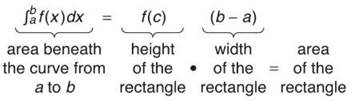
The Mean Value Theorem for Integration: If f(x) is a continuous function on the interval [a,b], then there exists a real number c on that interval such that
![]()
Translation: You can create a rectangle whose base is the interval and whose height is one of the function values in that interval. This is a very special rectangle because its area is exactly the same as the area beneath the curve on that interval.
Look at the graph of fix) below. If you count the boxes of area beneath it on the interval [1,9], you will get approximately 36.
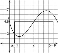
Also on the graph is a rectangle with length 9 — 1 = 8. It stretches across the interval at a height of 4.5, and its area is 36. Notice that f(c) = 4.5; this is the value promised by the MVTI. Let’s break down the parts of the theorem:
ALERT! Although the average value occurs at x = 5 in this example (and 5 is the mid point of [1,9]), the average value does not always occur at the midpoint of the interval.
The height of the rectangle, f(c), is also called the average value of f(x). In the example above, the average value is f(c) = 4.5. Imagine that the graph off(x) represents the flour in a measuring cup whose width is the interval [a,b].

If you shake the measuring cup back and forth, the flour will level out to its average height or average value. The resulting flour will have the same volume as the hillier version of it—it’s just flattened out. The same thing happens in two dimensions with the MVTI.
TIP. Make sure you memorize the average value formula. It is guaranteed to be on the test at least two or three times.
The AP test loves to ask questions about the average value of a function. Because of this, it helps to have the MVTI written in a different way—a way that lets you get right at the average value with no hassle. You get this formula quite easily; just multiply both sides of the MVTI by ![]() and you’ve got it.
and you’ve got it.
The Average Value of a Function: If f(x) is continuous on [a,b], the average value of the function, f(c), is given by
![]()
ALERT! 271/30 is a tiny bit more than 270/30 = 9, so in this case (although it was close), the average value is not halfway between the absolute maximum (12) and absolute minimum (6) for the closed interval. Some students assume that the average value always falls exactly in the middle.
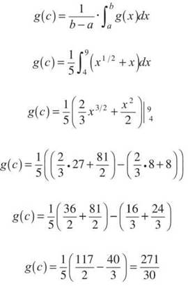
Example 9: Find the average value of the function g(x) = √x + x on [4,9].
Solution: The average value, g(c), will be given by
One final note before a parting example: Students sometimes get the average value of a function confused with the average rate of change of a function. Remember, the average value is based on definite integrals and is the “flour flattening” height of a function. The average rate of change is the slope of a secant line and describes rate over a period of time. Problem 4 following this section addresses this point of confusion.
Example 10: (a) Use your graphing calculator to find the average value of h(x) = x cos x on the interval [0,π].
We have no good techniques for integrating x cos x, and we’ll need to do so to find the average value of the function. The method is the same, but the means will be different:
![]()
Type the above directly into your calculator, using the “fnlnt” function found under the [Math] menu. If you do not know how to use your calculator to evaluate definite integrals, immediately read the technology section at the end of this chapter. The average value turns out to be h(c) = —.6366197724. In fact, the actual answer is —2/π.
(b) Find the c value guaranteed by the Mean Value Theorem for Integration.
The MVTI guarantees the existence of a c whose function value is the average value. In this problem, there is one input c whose output is —2/π; in other words, the point (c,—2/π) is on the graph of h(x). To find the c, plug the point into h(x):
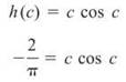
Solve this using your calculator, and you get: c = 1.911.
EXERCISE 6
NOTE. We have to integrate ∫ x cos x dx by parts. This is a BC-only topic.
Directions: Solve each of the following problems. Decide which is the best of the choices given and indicate your responses in the book.
YOU MAY USE YOUR CALCULATOR FOR PROBLEMS 3 AND 4 ONLY.
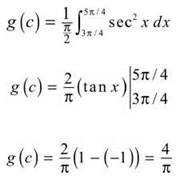
1. Find the average value of g(x) = sec2 x on the closed interval ![]()
2. If ![]() and
and ![]() what is the average value of f(x) on the interval [5,14]?
what is the average value of f(x) on the interval [5,14]?
NOTE. The MVTI guarantees that at least one such c will exist, but multiple c’s could be lurking around.
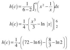
3. Find the value c guaranteed by the Mean Value Theorem for Integrals for the function ![]() on the interval [2,6].
on the interval [2,6].
4. A particle travels along the x-axis according to the position function ![]()
(a) What is the particle’s average velocity from t = π/2 to t = 2π?
(b) What is the velocity of the particle at any time t?
(c) Find the average value of the velocity function you found in part (b) on the interval ![]() and verify that you get the same result you did in part (a).
and verify that you get the same result you did in part (a).
ANSWERS AND EXPLANATIONS
1. The average value, g(c), is given by
2. First of all, you can rewrite the second definite integral as
![]()
Using another property of definite integrals, you know that
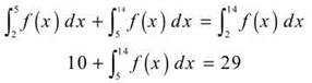
Therefore, ![]() With this value, you can complete the average value formula:
With this value, you can complete the average value formula:
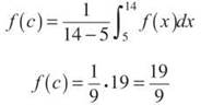
3. First, you should find the average value of the function:
Although this is the average value of the function, it is not the c guaranteed by the MVTI. However, if you plug c into h(x), you should get that result. Therefore,
![]()
Solve this with your graphing calculator to find that c ≈ 4.159.
4. (a) The average velocity is given by the slope of the secant line to a position function, just as the tangent lines to position functions give instantaneous velocity. The slope of the secant line is
(b) Since s is the position function, the velocity, v(t), is the derivative. Use the Product Rule (and the Chain Rule) to get
![]()
(c) Use your calculator’s fnlnt function to find the average value of v(t):
![]()
Therefore, you can find the average rate of change of a function two ways: (1) calculate the slope of the secant line of its original function, or (2) find a function that represents the rate of change and then calculate the average value of it. Pick your favorite technique. Collect ‘em and trade ‘em with your friends!