Master AP Calculus AB & BC
Part II. AP CALCULUS AB & BC REVIEW
CHAPTER 10. Differential Equations
HANDS-ON ACTIVITY 10.2: SLOPE FIELDS
Slope fields sound like dangerous places to play soccer but are, instead, handy ways to visualize differential equations. Remember back in the section on linear approximations when we discussed the fact that a derivative has values very close to its original function at the point of tangency? When that fact manifests itself all over the coordinate plane, it’s truly something to behold. So, you’d better be holding on to something when you undertake this activity.
1. Let’s return to the first differential equation from activity 10.1: ![]() . What exactly does this equation tell you about the general solution?
. What exactly does this equation tell you about the general solution?
________________________________________________________
2. If the solution to ![]() contained the point (0,1), what could you determine about the graph of the solution at that point?
contained the point (0,1), what could you determine about the graph of the solution at that point?
________________________________________________________
3. What would the tangent line to the solution graph look like at the point (—2,0)?
________________________________________________________
________________________________________________________
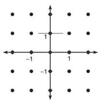
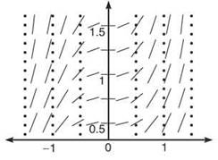
4. Calculate the slopes at all of the points indicated on the axes below, and draw a small line segment with the correct slope. The slope at point (0,1) has already been drawn as an example.
5. The general solution to ![]() (according to our work in the last chapter) was x2 + y2 = C. How does the solution relate to the drawing you made in problem 4?
(according to our work in the last chapter) was x2 + y2 = C. How does the solution relate to the drawing you made in problem 4?
________________________________________________________
________________________________________________________
6. What is the purpose of a slope field?
________________________________________________________
________________________________________________________
7. Draw the particular solution to ![]() that passes through the point (2,0) on the slope field above.
that passes through the point (2,0) on the slope field above.
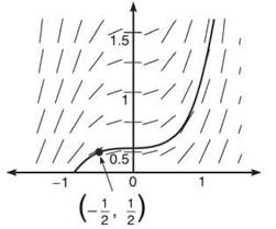
8. Draw the slope field for ![]() on the axes below.
on the axes below.
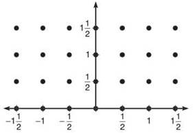
9. Use the slope field to draw an approximate solution graph that contains the point (-1/2,1/2).
10. Find the particular solution to ![]() that contains (-1/2,1/2) using separation of variables.
that contains (-1/2,1/2) using separation of variables.
________________________________________________________
________________________________________________________
________________________________________________________
11. Use your calculator to draw the graph of the particular solution you found in problem 10. It should look a lot like the graph you drew in problem 9.
SELECTED SOLUTIONS TO HANDS-ON ACTIVITY 10.2
Note: All slope fields in the solution are drawn with a computer and hence with more precision than in the exercises. Your slope fields should look similar, though not as detailed. See the technology section at the end of this chapter for a program to help you draw slope fields with your TI-83.
1. It tells you the slope, dy/dx, of the tangent lines to the solution graph at all points (x,y).
2. You would know that the slope of the tangent line to the graph at (0,1) would be ![]() The graph would have a horizontal tangent line there.
The graph would have a horizontal tangent line there.
3. The slope of the tangent line (also called the slope of the solution curve itself) is ![]() which is undefined. Therefore, the tangent line there is vertical (since a vertical line has an undefined slope).
which is undefined. Therefore, the tangent line there is vertical (since a vertical line has an undefined slope).
4. All you have to do is plug each (x,y) point into dy/dx to get the slope. Draw a small line segment with approximately that slope. It doesn’t have to be exact, but a slope of ½ should be much shallower than a slope of 2.
5. The tangent segments in the slope field trace out the circular shape of the solution graph. Remember that a tangent line has values very close to its original graph near the point of tangency. So, if we draw nothing but little tangent lines so small that all the points on the segment are close to the point of tangency, the result looks like the solution graph.
6. A slope field gives you a basic idea of the shape of the solution graph.
7. The particular solution will be a circle centered at the origin with radius 2.
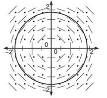
NOTE. The slope field actually looks like all the circles centered at the origin; that’s because a slope field doesn’t know the value of C, so it draws all possible circles.
8.
9.
10. Divide by y and multiply by dx to separate variables.
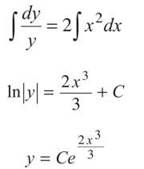
To find C, plug in the point (-1/2,1/2).
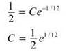
The final (unsimplified) solution is ![]()
EXERCISE 2
Directions: Solve each of the following problems. Decide which is the best of the choices given and indicate your responses in the book.
DO NOT USE A CALCULATOR FOR ANY OF THESE PROBLEMS.
1. Sketch the slope field of ![]()
2. (a) Draw the slope field for ![]()
(b) Find the solution of the differential equation that passes through the point (1,2e).
3. (a) Use the slope field of f'(x) = x/y to draw an approximate graph of f(x) if f(—2) = 0.
(b) Find/(x) specified in 3(a).
4. Explain how the slope field of ![]() describes its general solution.
describes its general solution.
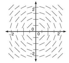
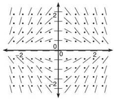
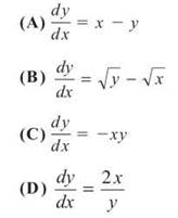
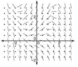
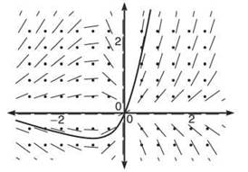
5. Which of the following differential equations has the slope field below?
ANSWERS AND EXPLANATIONS
1. All kinds of weird stuff happens close to the origin. Plot enough points so that you can see what’s going on. Remember, all you have to do is plug in any points (x,y) into the differential equation dy/dx; the result is the slope of the line segment you should draw at that point.
2. a)
(b) Solve the differential equation using separation of variables. You’ll have to factor a y out of the numerator to do so.
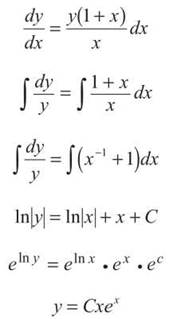
Now, plug in the point (1,2e).
2e = C(1)e
C = 2
Therefore, the solution is y = 2xex. If you graph it using your calculator (although the problem doesn’t ask you to do so), you’ll see that it fits the slope field perfectly.
3. (a) This slope field sort of looks like the big-bang theory—everything is exploding out of the origin. The solution just screams, “I am a hyperbola! Love me! Accept me! Tell me that I am handsome!”
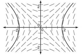
(b) It’s the revenge of separation of variables. In fact, this problem is very similar to the equation all of us are growing tired of: ![]() Begin by cross-multiplying.
Begin by cross-multiplying.
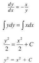
Now, find the C (Caspian).
0 = 4 + C
C = -4
All that remains is to plug in everything. Remember that the standard form for a hyberbola always equals 1.
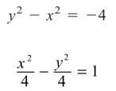
This is the equation of the hyberbola in part 3(a).
4. Elementary integration tells you that if ![]() , then y = x3 + C. The slope field for
, then y = x3 + C. The slope field for ![]() outlines the family of curves y = x3 + C.
outlines the family of curves y = x3 + C.
5. If you drew all four slope fields, you wasted valuable time; if this were the AP test, you’d have wasted five precious minutes on a very simple question in disguise. Look at the defining characteristic of the slope field: it has horizontal tangents all along thex- and y-axes. In other words, if either the y-coordinate of the point is 0 or the y-coordinate of the point is 0, then dy/dx equals 0. That is only true for one of the four choices: (C). For example, choice (D) is undefined at points that have y = 0; choices (A) and (B) won’t have horizontal tangents anywhere except for the origin.
NOTE. Euler is pronounced “oiler,” not “youler.”