5 Steps to a 5 AP Calculus AB & BC, 2012-2013 Edition (2011)

STEP 4. Review the Knowledge You Need to Score High

Chapter 10. Integration

IN THIS CHAPTER

Summary: On the AP Calculus exams, you will be asked to evaluate integrals of various functions. In this chapter, you will learn several methods of evaluating integrals including U-Substitution, Integration by Parts, and Integration by Partial Fractions. Also, you will be given a list of common integration and differentiation formulas, and a comprehensive set of practice problems. It is important that you work out these problems and check your solutions with the given explanations.

Key Ideas

Evaluating Integrals of Algebraic Functions

Integration Formulas

U-Substitution Method Involving Algebraic Functions

U-Substitution Method Involving Trigonometric Functions

U-Substitution Method Involving Inverse Trigonometric Functions

U-Substitution Method Involving Logarithmic and Exponential Functions

Integration by Parts

Integration by Partial Fractions

10.1 Evaluating Basic Integrals

Main Concepts: Antiderivatives and Integration Formulas, Evaluating Integrals

• Answer all parts of a question from Section II even if you think your answer to an earlier part of the question might not be correct. Also, if you do not know the answer to part one of a question, and you need it to answer part two, just make it up and continue.

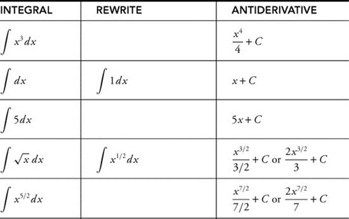
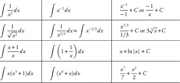
Antiderivatives and Integration Formulas

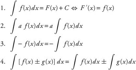
Definition: A function F is an antiderivative of another function f if F′(x) = f(x) for all x in some open interval. Any two antiderivatives of f differ by an additive constant C. We denote the set of antiderivatives of f by ∫ f(x)dx, called the indefinite integral of f.

Integration Rules:

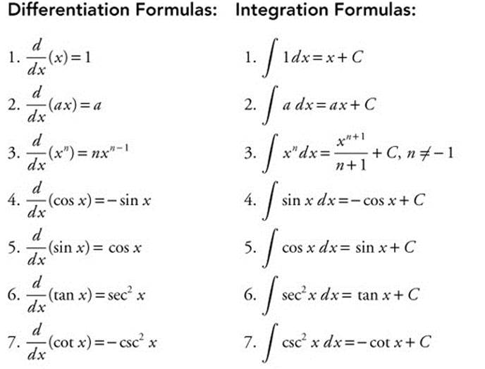
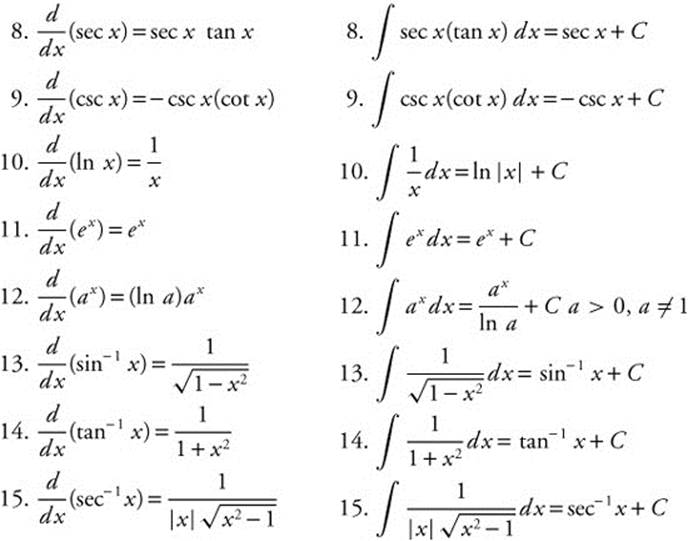
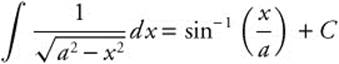
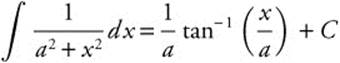
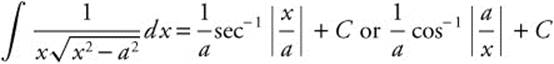
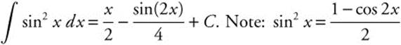
More Integration Formulas:

16. ∫ tan x dx = ln |sec x| + C or − ln |cos x | + C

17. ∫ cot x dx = ln |sin x| + C or − ln |csc x | + C

18. ∫ sec x dx = ln |sec x + tan x| + C

19. ∫ csc x dx = ln |csc x − cot x| + C

20. ∫ ln x dx = x ln |x| − x + C

21.

22.

23.

24.

Note: After evaluating an integral, always check the result by taking the derivative of the answer (i.e., taking the derivative of the antiderivative).

• Remember that the volume of a right-circular cone is where r is the radius of the base and h is the height of the cone.

Evaluating Integrals

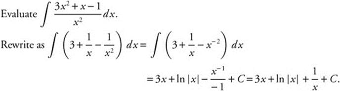
Example 1

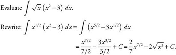
Example 2

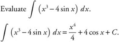
Example 3

If , and the point (0, −1) lies on the graph of y, find y.

Since , then y is an antiderivative of . Thus, y = ∫ (3_x² + 2) dx = x³ + 2x + C. The point (0, −1) is on the graph of y. Thus, y = x³ + 2x + C becomes −1 = 0³ + 2(0) + C or C = −1. Therefore, y = x³ + 2x − 1.

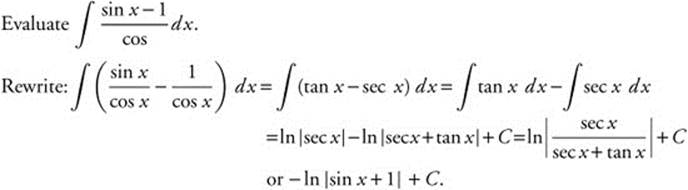
Example 4

Example 5

Example 6

Example 7

Example 8

Evaluate ∫ (4 cos x − cot x) dx.

∫ (4 cos x − cot x) dx = 4 sin x − ln |sin x| + C.

Example 9

Example 10

Example 11

Example 12

Example 13

Reminder: You can always check the result by taking the derivative of the answer.

• Be familiar with the instructions for the different parts of the exam before the day of exam. Review the instructions in the practice tests provided at the end of this book.

10.2 Integration by U-Substitution

Main Concepts:

The U-Substitution Method, U-Substitution and Algebraic Functions, U-Substitution and Trigonometric Functions, U-Substitution and Inverse Trigonometric Functions, U-Substitution and Logarithmic and Exponential Functions

The U-Substitution Method

The Chain Rule for Differentiation

, where F′ = f

The Integral of a Composite Function

If f(g(x)) and f′ are continuous and F′ = f, then

∫ f(g(x))g′(x)dx = F(g(x)) + C.

Making a U-Substitution

Let u = g(x), then du = g′(x)dx

∫ f(g(x))g″(x)dx = ∫ f(u)du = F(u) + C = F(g(x)) + C.

Procedure for Making a U-Substitution

Steps:

1. Given f(g(x)); let u = g(x).

2. Differentiate: du = g′(x)dx.

3. Rewrite the integral in terms of u.

4. Evaluate the integral.

5. Replace u by g(x).

6. Check your result by taking the derivative of the answer.

U-Substitution and Algebraic Functions

Another Form of the Integral of a Composite Function

If f is a differentiable function, then

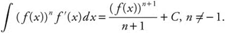
Making a U-Substitution

Let u = f(x); then du = f′(x)dx.

Example 1

Evaluate .

Step 1. Let u = x + 1; then x = u − 1.

Step 2. Differentiate: du = dx.

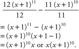
Step 3. Rewrite: .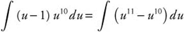

Step 4. Integrate: .

Step 5. Replace u: .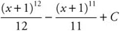

Step 6. Differentiate and Check:

Example 2

Evaluate .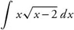

Step 1. Let u = x − 2; then x = u + 2.

Step 2. Differentiate: du = dx.

Step 3. Rewrite: .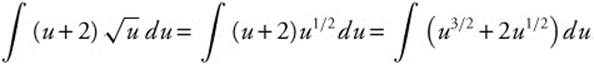

Step 4. Integrate: .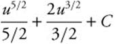

Step 5. Replace: .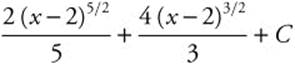

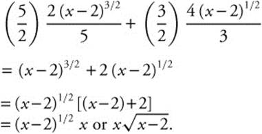
Step 6. Differentiate and Check:

Example 3

Evaluate .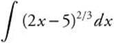

Step 1. Let u = 2x − 5.

Step 2. Differentiate: .

Step 3. Rewrite: .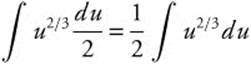

Step 4. Integrate: .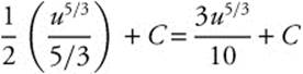

Step 5. Replace u: .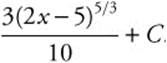

Step 6. Differentiate and Check: .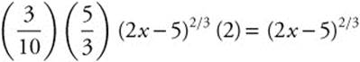

Example 4

Evaluate .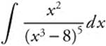

Step 1. Let u = x³ − 8.

Step 2. Differentiate: .

Step 3. Rewrite: .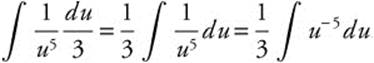

Step 4. Integrate: .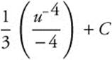

Step 5. Replace u: .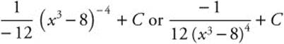

Step 6. Differentiate and Check: .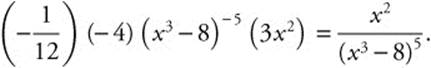

U-Substitution and Trigonometric Functions

Example 1

Evaluate .

Step 1. Let u = 4x.

Step 2. Differentiate: du = 4 dx or .

Step 3. Rewrite: .

Step 4. Integrate: .

Step 5. Replace u: .

Step 6. Differentiate and Check: .

Example 2

Evaluate .

Step 1. Let u = tan x.

Step 2. Differentiate: du = sec² x dx.

Step 3. Rewrite: .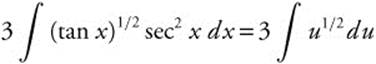

Step 4. Integrate: .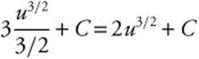

Step 5. Replace u: 2(tan x)^3/2 + C or 2 tan^3/2 x + C.

Step 6. Differentiate and Check: .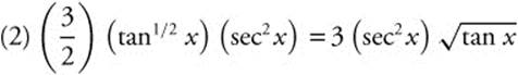

Example 3

Evaluate .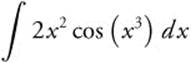

Step 1. Let u = x³.

Step 2. Differentiate: .

Step 3. Rewrite: .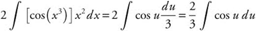

Step 4. Integrate: .

Step 5. Replace u: .

Step 6. Differentiate and Check: .

• Remember that the area of a semi-circle is . Do not forget the . If the cross sections of a solid are semi-circles, the integral for the volume of the solid will involve which is .

U-Substitution and Inverse Trigonometric Functions

Example 1

Evaluate .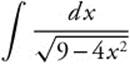

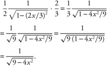
Step 1. Let u = 2x.

Step 2. Differentiate: .

Step 3. Rewrite: .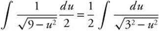

Step 4. Integrate: .

Step 5. Replace u: .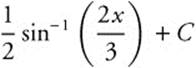

Step 6. Differentiate and Check:

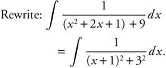
Example 2

Evaluate .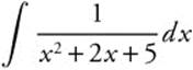

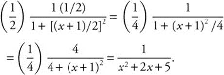
Step 1. Rewrite:

.

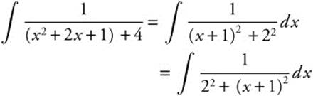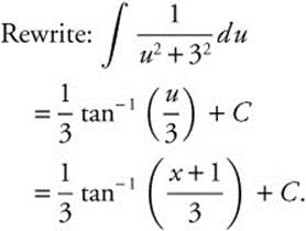
Let u = x + 1.

Step 2. Differentiate: du = dx.

Step 3. Rewrite: .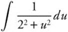

Step 4. Integrate: .

Step 5. Replace u: .

Step 6. Differentiate and Check:

• If the problem gives you that the diameter of a sphere is 6 and you are using formulas such as or s = 4π r², do not forget that r = 3.

U-Substitution and Logarithmic and Exponential Functions

Example 1

Evaluate .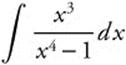

Step 1. Let u = x⁴ − 1.

Step 2. Differentiate: .

Step 3. Rewrite: .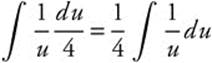

Step 4. Integrate: .

Step 5. Replace u: .

Step 6. Differentiate and Check: .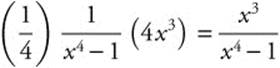

Example 2

Evaluate .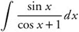

Step 1. Let u = cos x + 1.

Step 2. Differentiate: du = −sin xdx ⇒ − du = sin xdx.

Step 3. Rewrite: .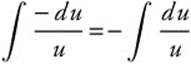

Step 4. Integrate: − ln |u| + C.

Step 5. Replace u: − ln |cos x + 1| + C.

Step 6. Differentiate and Check: .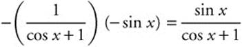

Example 3

Evaluate .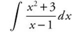

Step 1. Rewrite ; by dividing (x² + 3) by (x − 1).

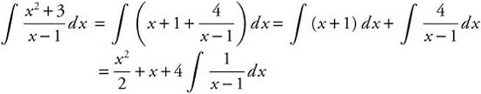
Let u = x − 1.

Step 2. Differentiate: du = dx.

Step 3. Rewrite: .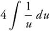

Step 4. Integrate: 4 ln |u| + C.

Step 5. Replace u: 4 ln |x − 1| + C.

.

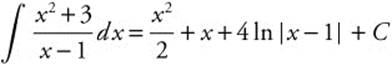Step 6. Differentiate and Check:

.

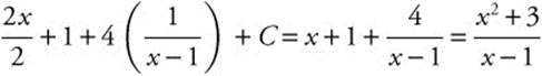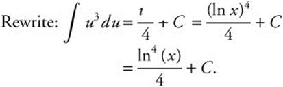
Example 4

Evaluate .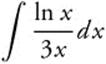

Step 1. Let u = ln x.

Step 2. Differentiate: .

Step 3. Rewrite: .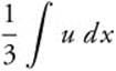

Step 4. Integrate: .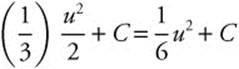

Step 5. Replace u: .

Step 6. Differentiate and Check: .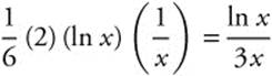

Example 5

Evaluate .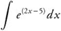

Step 1. Let u = 2x − 5.

Step 2. Differentiate: .

Step 3. Rewrite: .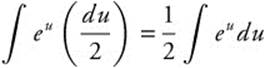

Step 4. Integrate: .

Step 5. Replace u: .

Step 6. Differentiate and Check: .

Example 6

Evaluate .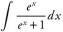

Step 1. Let u = e^x + 1.

Step 2. Differentiate: du = e^xdx.

Step 3. Rewrite: .

Step 4. Integrate: ln |u| + C.

Step 5. Replace u: ln |e^x + 1| + C.

Step 6. Differentiate and Check: .

Example 7

Evaluate .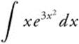

Step 1. Let u = 3x².

Step 2. Differentiate: .

Step 3. Rewrite: .

Step 4. Integrate: .

Step 5. Replace u: .

Step 6. Differentiate and Check: .

Example 8

Evaluate .

Step 1. Let u = 2x.

Step 2. Differentiate: .

Step 3. Rewrite: .

Step 4. Integrate: .

Step 5. Replace u: .

Step 6. Differentiate and Check: (5^2x)(2) ln 5/2 ln 5 = 5^2x.

Example 9

Evaluate .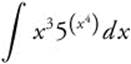

Step 1. Let u = x⁴.

Step 2. Differentiate: .

Step 3. Rewrite: .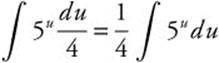

Step 4. Integrate: .

Step 5. Replace u: .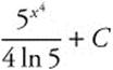

Step 6. Differentiate and Check: .

Example 10

Evaluate .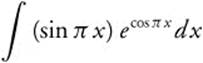

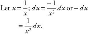
Step 1. Let u = cos π x.

Step 2. Differentiate: du = −π sin π x dx; .

Step 3. Rewrite: .

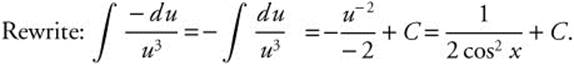
Step 4. Integrate: .

Step 5. Replace u: .

Step 6: Differentiate and Check: .

10.3 Techniques of Integration

Main Concepts: Integration by Parts, Integration by Partial Fractions

Integration by Parts

According to the product rule for differentiation . Integrating tells us that 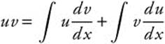, and therefore 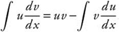. To integrate a product, careful identification of one factor as u and the other as allows the application of this rule for integration by parts. Choice of one factor to be u (and therefore the other to be dv) is simpler if you remember the mnemonic LIPET. Each letter in the acronym represents a type of function: Logarithmic, Inverse trigonometric, Polynomial, Exponential, and Trigonometric. As you consider integrating by parts, assign the factor that falls earlier in the LIPET list as u, and the other as dv.

Example 1

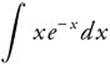
Step 1: Identify u = x and dv = e^−x dx since x is a Polynomial, which comes before Exponential in LIPET.

Step 2: Differentiate du = dx and integrate v = −e^−x.

Step 3: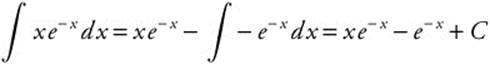

Example 2

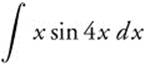
Step 1: Identify u = x and dv = sin 4x dx since x is a Polynomial, which comes before Trigonometric in LIPET.

Step 2: Differentiate du = dx and integrate .

Step 3:

Integration by Partial Fractions

A rational function with a factorable denominator can be integrated by decomposing the integrand into a sum of simpler fractions. Each linear factor of the denominator becomes the denominator of one of the partial fractions.

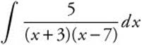
Example 1

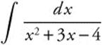
Step 1: Factor the denominator: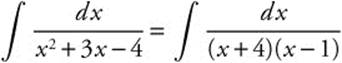

Step 2: Let A and B represent the numerators of the partial fractions .

Step 3: The algorithm for adding fractions tells us that A(x − 1) + B(x + 4) = 1, so Ax + Bx = 0 and − A + 4B = 1. Solving gives us A = −0.2 and B = 0.2.

Step 4: 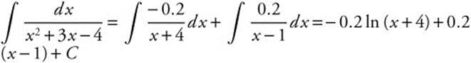ln

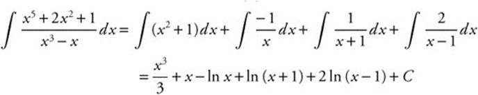
Example 2

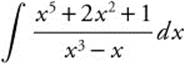
Step 1: Use long division to rewrite .

Step 2: Factor the denominator: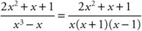

Step 3: Let A, B, and C represent the numerators of the partial fractions.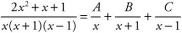

Step 4: 2x² + x + 1 = A(x + 1)(x − 1) + Bx(x − 1) + Cx(x + 1), therefore, Ax² + Bx² + Cx² = 2x², Cx − Bx = x, and −A = 1. Solving gives A = −1, B = 1, and C = 2.

Step 5:

10.4 Rapid Review

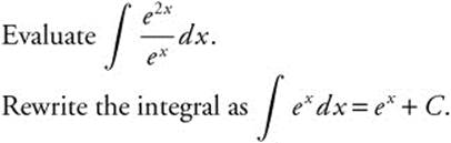
1. Evaluate .

Answer: Rewrite as .

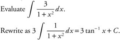
2. Evaluate .

Answer: Rewrite as .

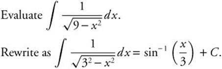
3. Evaluate .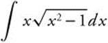

Answer: Rewrite as .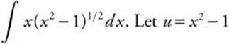

Thus, .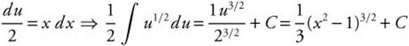

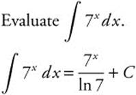
4. Evaluate .

Answer: −cos x + C.

5. Evaluate .

Answer: Let u = 2x and obtain .

6. Evaluate .

Answer: Let u = ln x; and obtain .

7. Evaluate .

Answer: Let u = x²; and obtain .

8.

Answer: Let u = x, du = dx, dv = cos xdx, and v = sin x, then .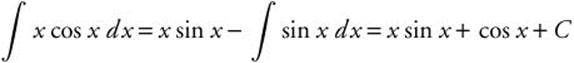

9.

Answer:

10.5 Practice Problems

Evaluate the following integrals in problems 1 to 20. No calculators are allowed. (However, you may use calculators to check your results.)

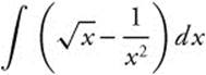
1.

2.

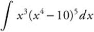
3.

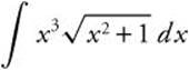
4.

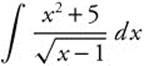
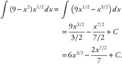
5.

6.

7.

8.

9.

10.

11.

12.

13.

14.

15.

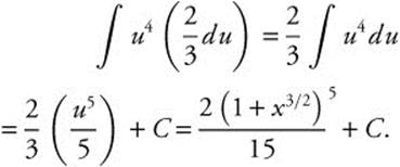
16.

17. If and the point (0, 6) is on the graph of y, find y.

18.

19.

20. If f(x) is the antiderivative of and f(1) = 5, find f(e).

21.

22.

23.

24.

25.

10.6 Cumulative Review Problems

(Calculator) indicates that calculators are permitted.

26. The graph of the velocity function of a moving particle for 0 ≤ t ≤ 10 is shown in Figure 10.6-1.

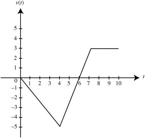
Figure 10.6-1

(a) At what value of t is the speed of the particle the greatest?

(b) At what time is the particle moving to the right?

27. Air is pumped into a spherical balloon, whose maximum radius is 10 meters. For what value of r is the rate of increase of the volume a hundred times that of the radius?

28. Evaluate .

29. (Calculator) The function f is continuous and differentiable on (0, 2) with f″(x) > 0 for all x in the interval (0, 2). Some of the points on the graph are shown below.

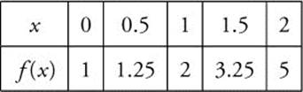
Which of the following is the best approximation for f′(1)?

(a) f′(1) < 2

(b) 0.5 < f′(1) < 1

(c) 1.5 < f′(1) < 2.5

(d) 2.5 < f′(1) < 3.5

(e) f′(1) > 2

30. The graph of the function f″ on the interval [1, 8] is shown in Figure 10.6-2. At what value(s) of t on the open interval (1, 8), if any, does the graph of the function f′:

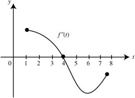
Figure 10.6-2

(a) have a point of inflection?

(b) have a relative maximum or minimum?

(c) become concave upward?

31. Evaluate .

32. If the position of an object is given by x = 4 sin(πt), y = t² − 3t + 1, find the position of the object at t = 2.

33. Find the slope of the tangent line to the curve r = 3 cos θ when .

10.7 Solutions to Practice Problems

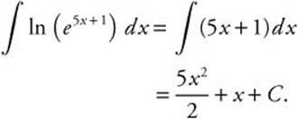
1.

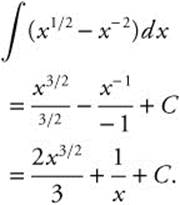
2. Rewrite:

3. Let u = x⁴ − 10du = 4x³dx or .

Rewrite

.

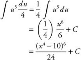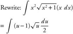
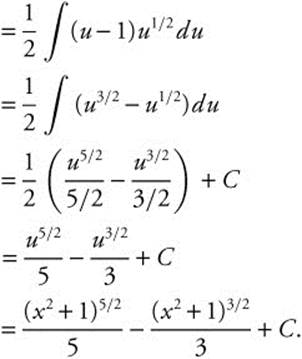
4. Let u = x² + 1 ⇒ (u − 1) = x² and du = 2x dx or .

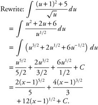
5. Let u = x − 1; du = dx and (u + 1) = x.

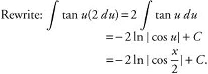
6. Let ; or 2du = dx.

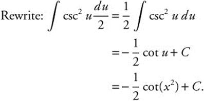
7. Let u = x²; du = 2x dx or .

8. Let u = cos x; du = −sin x dx or −du = sin x dx.

9.

Let u = x + 1; du = dx.

10.

11. Rewrite: .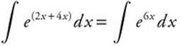

Let u = 6x; du = 6 dx or .

12. Let u = ln x; .

13. Since e^x and ln x are inverse functions:

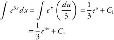
14.

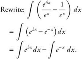
Let u = 3x; du = 3dx;

Let v = −x; dv = −dx;

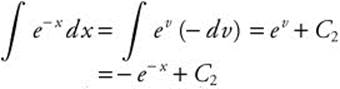
Thus .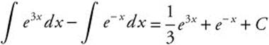

Note: C₁ and C₂ are arbitrary constants, and thus C₁ + C₂ = C.

15. Rewrite:

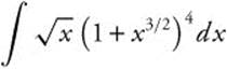
16. Let u = 1 + x^3/2; or .

Rewrite:

17. Since , then y = .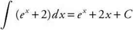

The point (0, 6) is on the graph of y. Thus, 6 = e⁰ + 2(0) + C ⇒ 6 = 1 + C or C = 5. Therefore, y = e^x + 2x + 5.

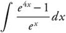
18. Let u = e^x; du = e^x dx.

Rewrite: −3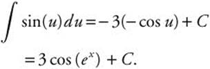

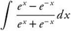
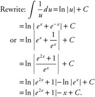
19. Let u = e^x + e^−x; du = (e^x − e^−x) dx.

20. Since f(x) is the antiderivative of , .

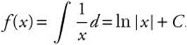Given f(1) = 5; thus, ln (1) + C = 5 ⇒ 0 + C = 5 or C = 5.

Thus, f(x) = ln |x| + 5 and f(e) = ln (e) + 5 = 1 + 5 = 6.

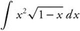
21. Integrate 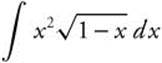by parts. Let u = x², du = 2x dx, , and . Then 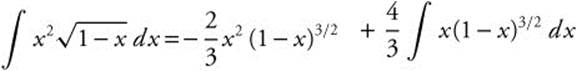. Use parts again with u = x, du = dx, dv= (1 − x)^3/2 dx, and so that 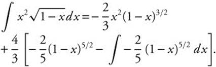. Integrate for and simplify to .

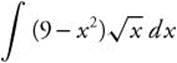
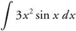
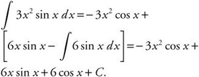
22. For 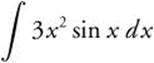, use integration by parts with u = 3x², du = 6x dx, dv = sin x dx, and v = −cos x.

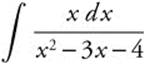
23. Factor the denominator so that 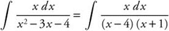. Use a partial fraction decomposition, 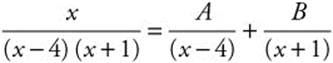, which implies Ax + A + Bx − 4B = x. Solve A + B = 1 and A − 4B to find and . Integrate .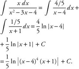

24. Factor 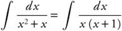and use partial fractions. If 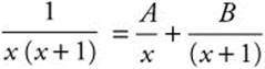, Ax + A + Bx = 1 and A = −B = 1.

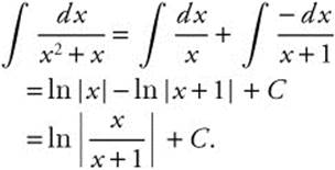
25. Begin with integration by parts, using u = ln x, , , 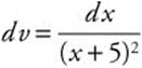and .

Then

.

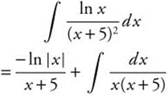Use a partial fraction decomposition 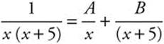. Solve to find . Then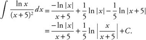

10.8 Solutions to Cumulative Review Problems

26. (a) At t = 4, speed is 5 which is the greatest on 0 ≤ t ≤ 10.

(b) The particle is moving to the right when 6 < t < 10.

27.

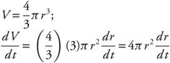
If , then .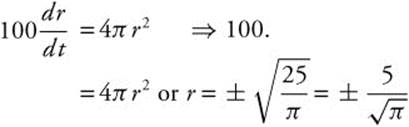

Since r ≥ 0, meters.

28. Let u = ln x; .

29. Label given points as A, B, C, D, and E. Since f″(x) > 0 ⇒ f is concave upward for all x in the interval [0, 2]. Thus, and . Therefore, 1.5 < f′(1) < 2.5, choice (c). (See Figure 10.8-1.)

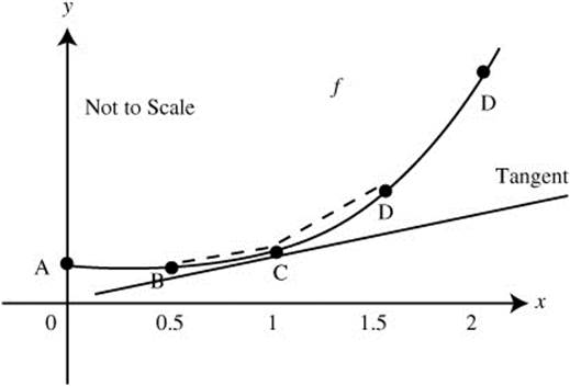
Figure 10.8-1

30. (a) f″ is decreasing on [1, 6) ⇒ f″′< 0 ⇒ f′ is concave downward on [1, 6) and f″ is increasing on (6, 8] ⇒ f′ is concave upward on (6, 8]. Thus, at x = 6, f′ has a change of concavity. Since f″ exists at x = 6 (which implies there is a tangent to the curve of f′ at x = 6), f′ has a point of inflection at x = 6.

(b) f″ > 0 on [1, 4] ⇒ f′ is increasing and f″ < 0 on (4, 8] ⇒ f′ is decreasing. Thus at x = 4, f′ has a relative maximum at x = 4. There is no relative minimum.

(c) f″ is increasing on [6, 8] ⇒ f′ > 0 ⇒ f′ is concave upward on [6, 8].

31.

32. At t = 2, x = 4 sin(2π) = 0, and , so the position of the object at t = 2 is (0, −1).

33. To find the slope of the tangent line to the curve r = 3 cos θ when , begin with x = r cos θ and y = r sinθ, and find and so . y = 3 cos θ sinθ so . Then the slope of the tangent line is . . Evaluate at to get . The slope of the tangent line is zero, indicating that the tangent is horizontal.