5 Steps to a 5: AP Calculus AB 2017 (2016)

STEP 4

Review the Knowledge You Need to Score High

CHAPTER 10

Big Idea 2: Derivatives

More Applications of Derivatives

IN THIS CHAPTER

Summary : Finding an equation of a tangent is one of the most common questions on the AP Calculus AB exam. In this chapter, you will learn how to use derivatives to find an equation of a tangent, and to use the tangent line to approximate the value of a function at a specific point. You will also learn to apply derivatives to solve rectilinear motion problems.

Key Ideas

Tangent and Normal Lines

Linear Approximations

Motion Along a Line

10.1 Tangent and Normal Lines

Main Concepts: Tangent Lines, Normal Lines

Tangent Lines

If the function y is differentiable at x = a , then the slope of the tangent line to the graph of y at x = a is given as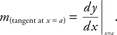

Types of Tangent Lines

Horizontal Tangents: . (See Figure 10.1-1 .)

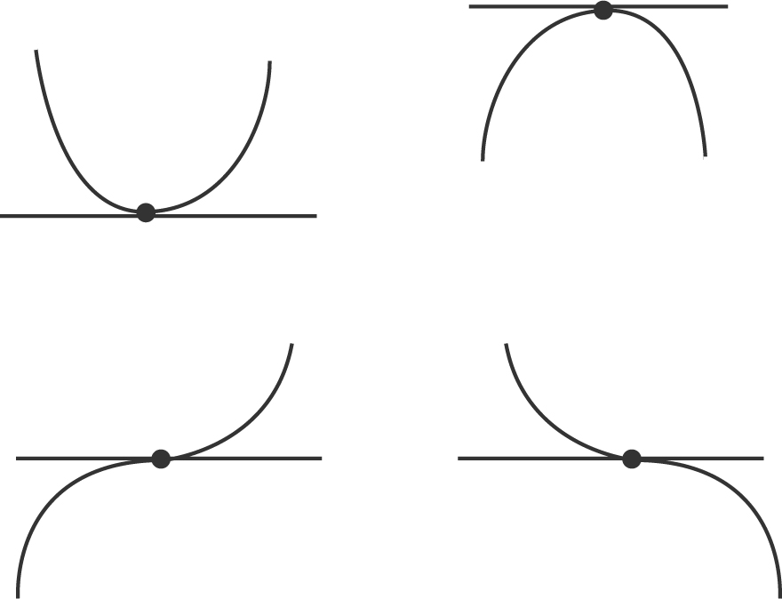
Figure 10.1-1

Vertical Tangents: ( does not exist but = 0). (See Figure 10.1-2 .)

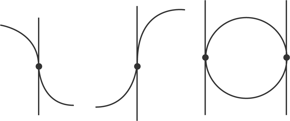
Figure 10.1-2

Parallel Tangents: . (See Figure 10.1-3 .)

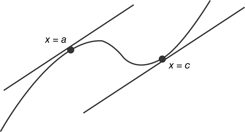
Figure 10.1-3

Example 1

Write an equation of the line tangent to the graph of y = –3 sin 2x at . (See Figure 10.1-4 .)

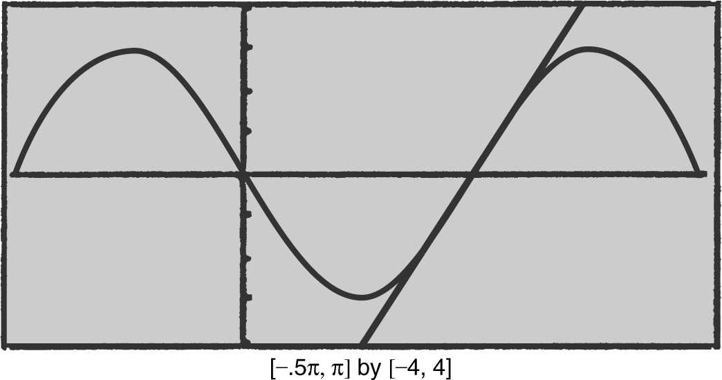
Figure 10.1-4

y = –3 sin 2x ;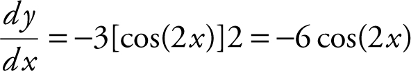

Slope of tangent .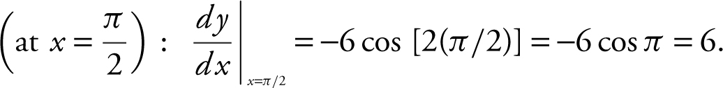

Point of tangency: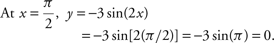

Therefore, is the point of tangency.

Equation of tangent: y – 0 = 6(x – π /2) or y = 6x – 3π .

Example 2

If the line y = 6x + a is tangent to the graph of y = 2x ³ , find the value(s) of a .

Solution:

(See Figure 10.1-5 .)

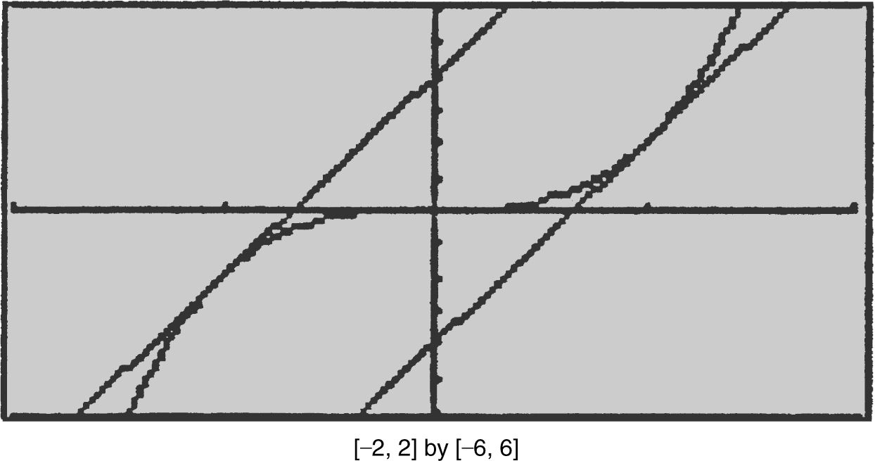
Figure 10.1-5

The slope of the line y = 6x + a is 6.

Since y = 6x + a is tangent to the graph of y = 2x ³ , thus 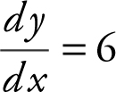for some values of x .

Set 6x ² = 6 ⇒ x ² = 1 or x = ±1.

At x = –1, y = 2x ³ = 2(–1)³ = –2;(–1, –2) is a tangent point. Thus, y = 6x + a ⇒ –2 = 6(–1) + a or a = 4.

At x = 1, y = 2x ³ = 2(1)³ = 2; (1, 2) is a tangent point.

Thus, y = 6x + a ⇒ 2 = 6(1) + a or a = –4.

Therefore, a = ±4.

Example 3

Find the coordinates of each point on the graph of y ² – x ² – 6x + 7 = 0 at which the tangent line is vertical. Write an equation of each vertical tangent. (See Figure 10.1-6 .)

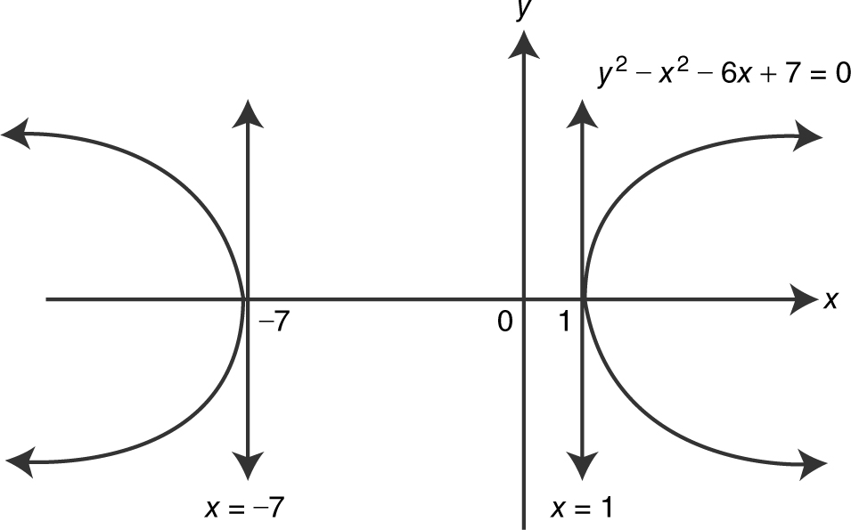
Figure 10.1-6

Step 1: Find .

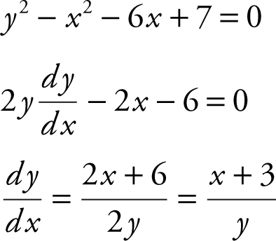
Step 2: Find .

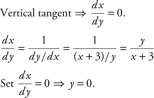
Step 3: Find points of tangency.

At y = 0, y ² – x ² – 6x + 7 = 0 becomes –x ² – 6x + 7 = 0 ⇒ x ² + 6x – 7 = 0 ⇒ (x + 7)(x – 1) = 0 ⇒ x = –7 or x = 1.

Thus, the points of tangency are (–7, 0) and (1, 0).

Step 4: Write equations for vertical tangents: x = –7 and x = 1.

Example 4

Find all points on the graph of y = |xe^x | at which the graph has a horizontal tangent.

Step 1: Find .

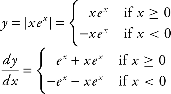
Step 2: Find the x -coordinate of points of tangency.

Horizontal tangent .

If x ≥ 0, set e^x + xe^x = 0 ⇒ e^x (1 + x ) = 0 ⇒ x = –1 but x ≥ 0, therefore, no solution.

If x < 0, set –e^x – xe^x = 0 ⇒ –e^x (1 + x ) = 0 ⇒ x = –1.

Step 3: Find points of tangency.

At

Thus at the point (–1, 1/e ), the graph has a horizontal tangent. (See Figure 10.1-7 .)

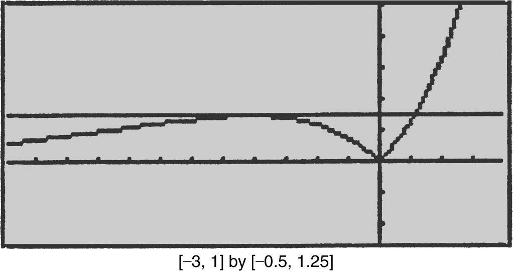
Figure 10.1-7

Example 5

Using your calculator, find the value(s) of x to the nearest hundredth at which the slope of the line tangent to the graph of y = 2 ln (x ² + 3) is equal to . (See Figures 10.1-8 and 10.1-9 .)

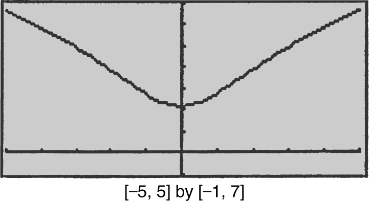
Figure 10.1-8

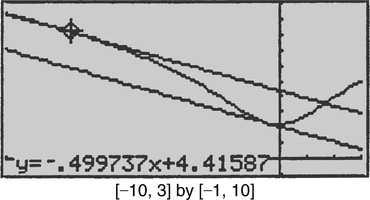
Figure 10.1-9

Step 1: Enter y 1 = 2 ∗ ln (x ^2 + 3).

Step 2: Enter y 2 = d (y ₁ (x ), x ) and enter

Step 3: Using the [Intersection ] function of the calculator for y ₂ and y ₃ , you obtain x = –7.61 or x = –0.39.

Example 6

Using your calculator, find the value(s) of x at which the graphs of y = 2x ² and y = e^x have parallel tangents.

Step 1: Find for both y = 2x ² and y = e^x .

Step 2: Find the x -coordinate of the points of tangency. Parallel tangents ⇒ slopes are equal.

Set 4x = e^x ⇒ 4x – e^x = 0.

Using the [Solve ] function of the calculator, enter [Solve ] (4x – e ^(x ) = 0, x ) and obtain x = 2.15 and x = 0.36.

• Watch out for different units of measure, e.g., the radius, r , is 2 feet, find in inches per second.

Normal Lines

The normal line to the graph of f at the point (x ₁ , y ₁ ) is the line perpendicular to the tangent line at (x ₁ , y ₁ ). (See Figure 10.1-10 .)

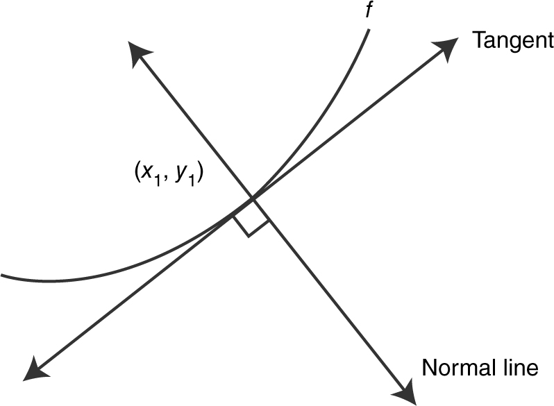
Figure 10.1-10

Note that the slope of the normal line and the slope of the tangent line at any point on the curve are negative reciprocals, provided that both slopes exist.

(m _{normal line} )(m _{tangent line} ) = –1.

Special Cases:
(See Figure 10.1-11 .)

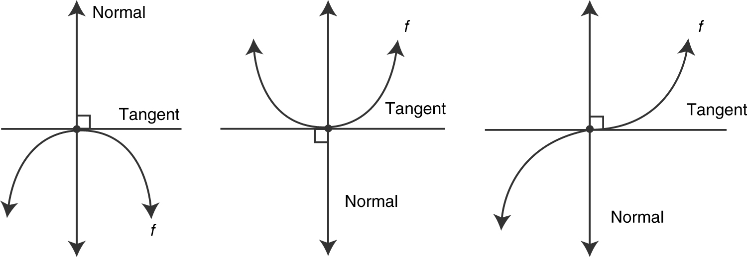
Figure 10.1-11

At these points, m _tangent = 0; but m _normal does not exist.

(See Figure 10.1-12 .)

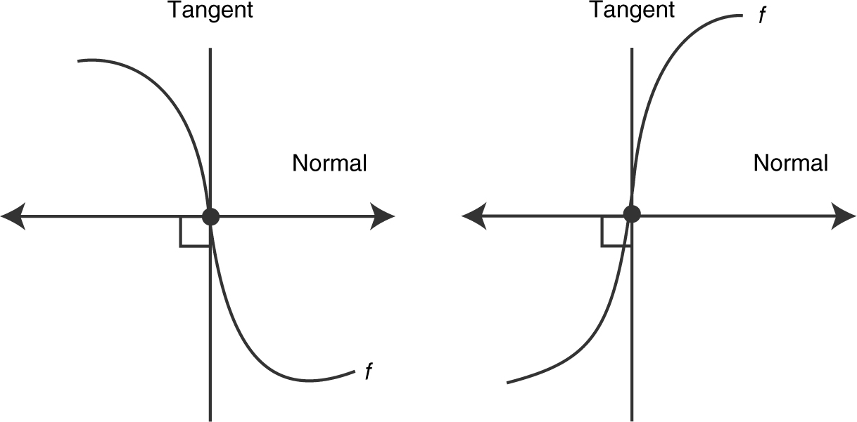
Figure 10.1-12

At these points, m _tangent does not exist; however m _normal = 0.

Example 1

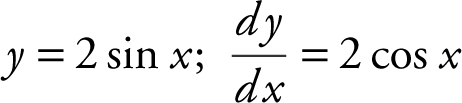
Write an equation for each normal to the graph of y = 2 sin x for 0 ≤ x ≤ 2π that has a slope of .

Step 1: Find m _tangent .

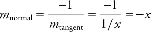
Step 2: Find m _normal .

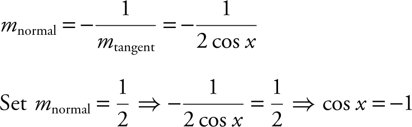
⇒ x = cos^–1 (–1) or x = π . (See Figure10.1-13 .)

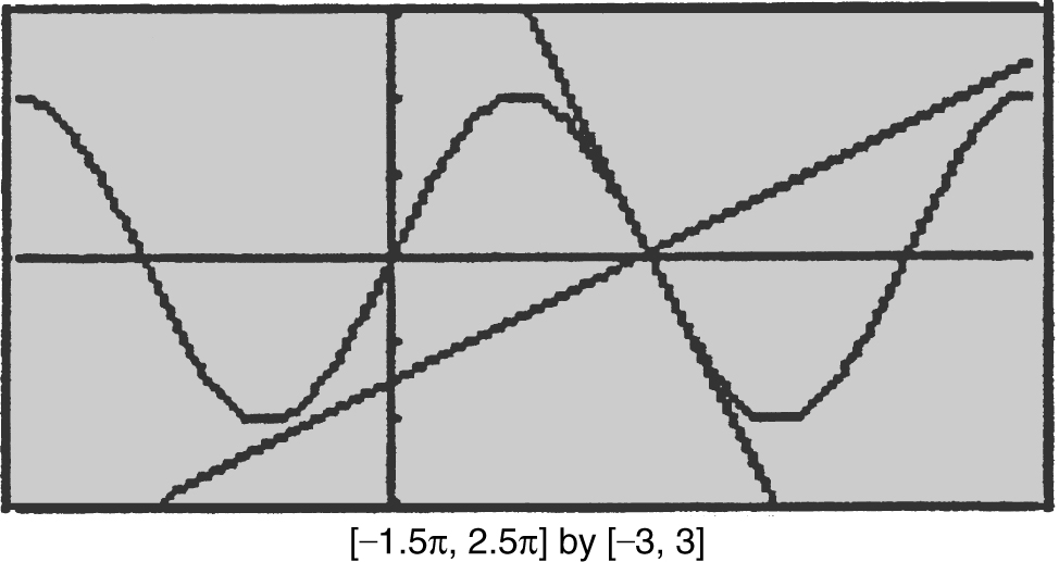
Figure 10.1-13

Step 3: Write equation of normal line.

At x = π , y = 2 sin x = 2(0) = 0; (π , 0).

Since , equation of normal is:

or .

Example 2

Find the point on the graph of y = ln x such that the normal line at this point is parallel to the line y = –ex – 1.

Step 1: Find m _tangent .

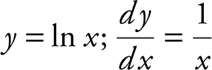
Step 2: Find m _normal .

Slope of y = –ex – 1 is –e .

Since normal is parallel to the line y = –ex – 1, set m _normal = –e ⇒ –x = –e or x = e .

Step 3: Find the point on the graph. At x = e , y = ln x = ln e = l . Thus the point of the graph of y = ln x at which the normal is parallel to y = –ex – 1 is (e , 1). (See Figure 10.1-14 .)

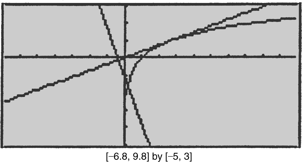
Figure 10.1-14

Example 3

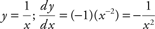
Given the curve : (a) write an equation of the normal to the curve at the point (2, 1/2), and (b) does this normal intersect the curve at any other point? If yes, find the point.

Step 1: Find m _tangent .

Step 2: Find m _normal .

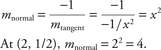
Step 3: Write equation of normal.

m _normal = 4; (2, 1/2)

Equation of normal: , or .

Step 4: Find other points of intersection.

Using the [Intersection ] function of your calculator, enter and and obtain x = –0.125 and y = –8. Thus, the normal line intersects the graph of at the point (–0.125, –8) as well.

• Remember that and .

10.2 Linear Approximations

Main Concepts: Tangent Line Approximation, Estimating the n th Root of a Number, Estimating the Value of a Trigonometric Function of an Angle

Tangent Line Approximation (or Linear Approximation)

An equation of the tangent line to a curve at the point (a , f (a )) is: y = f (a ) + f ′ (a )(x – a ), providing that f is differentiable at a . (See Figure 10.2-1 .) Since the curve of f (x ) and the tangent line are close to each other for points near x = a , f (x ) ≈ f (a ) + f ′ (a )(x – a ).

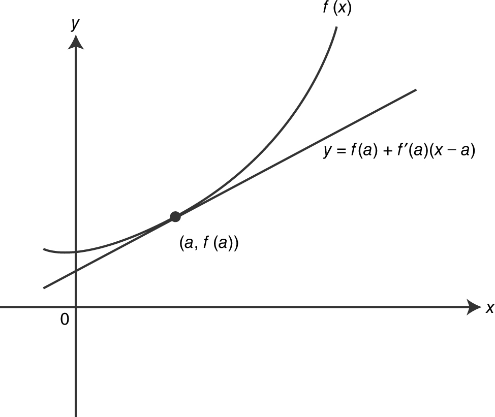
Figure 10.2-1

Example 1

Write an equation of the tangent line to f (x ) = x ³ at (2, 8). Use the tangent line to find the approximate values of f (1.9) and f (2.01).

Differentiate f (x ): f ′(x ) = 3x ² ; f ′(2) = 3(2)² = 12. Since f is differentiable at x = 2, an equation of the tangent at x = 2 is:

y = f (2) + f ′ (2)(x – 2)
y = (2)³ + 12(x – 2) = 8 + 12x – 24 = 12x – 16
f (1.9) ≈ 12(1.9) – 16 = 6.8
f (2.01) ≈ 12(2.01) – 16 = 8.12. (See Figure 10.2-2 .)

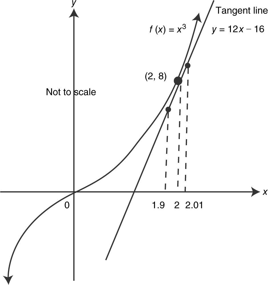
Figure 10.2-2

Example 2

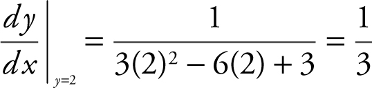
If f is a differentiable function and f (2) = 6 and , find the approximate value of f (2.1).

Using tangent line approximation, you have

(a) f (2) = 6 ⇒ the point of tangency is (2, 6);

(b) ⇒ the slope of the tangent at x = 2 is ;

(c) the equation of the tangent is or ;

(d) thus, .

Example 3

The slope of a function at any point (x , y ) is . The point (3, 2) is on the graph of f . (a) Write an equation of the line tangent to the graph of f at x = 3. (b) Use the tangent line in part (a) to approximate f (3.1).

(a) Let y = f (x ), then

Equation of tangent: y – 2 = –2(x – 3) or y = –2x + 8.

(b) f (3.1) ≈ –2(3.1) + 8 ≈ 1.8

Estimating the n th Root of a Number

Another way of expressing the tangent line approximation is: f (a + Δx ) ≈ f (a ) + f ′(a )Δx , where Δx is a relatively small value.

Example 1

Find the approximate value of using linear approximation.

Using and Δx = 1.

Thus,

Example 2

Find the approximate value of using linear approximation.

Let f (x ) = x ^1/3 , a = 64, Δx = – 2. Since and , you can use f (a + Δx ) ≈ f (a ) + f ′(a )Δx . Thus, f (62) =

• Use calculus notations and not calculator syntax, e.g., write and not .

Estimating the Value of a Trigonometric Function of an Angle

Example

Approximate the value of sin 31°.

Note: You must express the angle measurement in radians before applying linear approximations. radians and radians.

Let f (x ) = sin x , and .

Since f ′ (x ) = cos x and , you can use linear approximations:

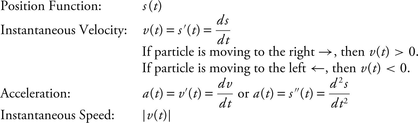
10.3 Motion Along a Line

Main Concepts: Instantaneous Velocity and Acceleration, Vertical Motion, Horizontal Motion

Instantaneous Velocity and Acceleration

Example 1

The position function of a particle moving on a straight line is s (t ) = 2t ³ – 10t ² + 5. Find (a) the position, (b) instantaneous velocity, (c) acceleration, and (d) speed of the particle at t = 1.

Solution:

(a) s (1) = 2(1)³ – 10(1)² + 5 = –3

(b) v (t ) = s ′(t ) = 6t ² – 20t
v (1) = 6(1)² – 20(1) = –14

(c) a (t ) = v ′(t ) = 12t – 20
a (1) = 12(1) – 20 = –8

(d) Speed = |v (t )| = |v (1)| = 14

Example 2

The velocity function of a moving particle is 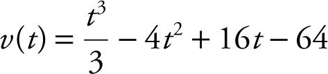for 0 ≤ t ≤ 7.

What is the minimum and maximum acceleration of the particle on 0 ≤ t ≤ 7?

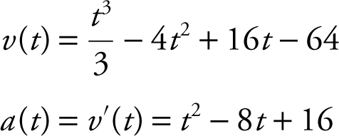
(See Figure 10.3-1 .) The graph of a (t ) indicates that:

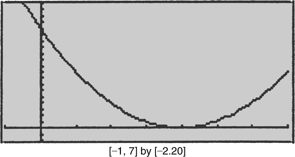
Figure 10.3-1

(1) The minimum acceleration occurs at t = 4 and a (4) = 0.

(2) The maximum acceleration occurs at t = 0 and a (0) = 16.

Example 3

The graph of the velocity function is shown in Figure 10.3-2 .

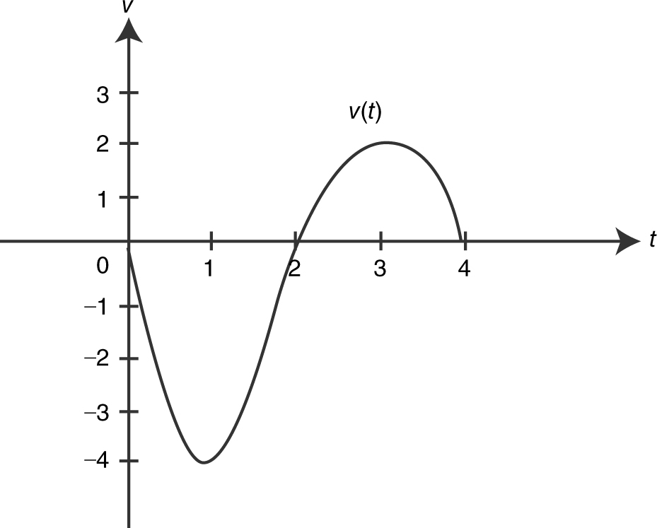
Figure 10.3-2

(a) When is the acceleration 0?

(b) When is the particle moving to the right?

(c) When is the speed the greatest?

Solution:

(a) a (t ) = v ′(t ) and v ′(t ) is the slope of tangent to the graph of v . At t = 1 and t = 3, the slope of the tangent is 0.

(b) For 2 < t < 4, v (t ) > 0. Thus the particle is moving to the right during 2 < t < 4.

(c) Speed = |v (t )| at t = 1, v (t ) = –4.
Thus, speed at t = 1 is |–4| = 4 which is the greatest speed for 0 ≤ t ≤ 4.

• Use only the four specified capabilities of your calculator to get your answer: plotting graphs, finding zeros, calculating numerical derivatives, and evaluating definite integrals. All other built-in capabilities can only be used to check your solution.

Vertical Motion

Example

From a 400-foot tower, a bowling ball is dropped. The position function of the bowling ball s (t ) = –16t ² + 400, t ≥ 0 is in seconds. Find:

(a) the instantaneous velocity of the ball at t = 2 seconds.

(b) the average velocity for the first 3 seconds.

(c) when the ball will hit the ground.

Solution:

(a) v (t ) = s ′(t ) = –32t
v (2) = 32(2) = –64 ft/sec

(b) Average velocity .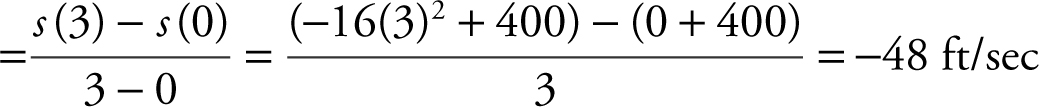

(c) When the ball hits the ground, s (t ) = 0.
Thus, set s (t ) = 0 ⇒ –16t ² + 400 = 0; 16t ² = 400; t = ±5.
Since t ≥ 0, t = 5. The ball hits the ground at t = 5 sec.

• Remember that the volume of a sphere is 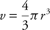and the surface area is s = 4πr ² . Note that v ′ = s .

Horizontal Motion

Example

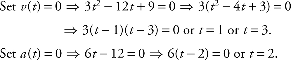
The position function of a particle moving in a straight line is s (t ) = t ³ – 6t ² + 9t – 1, t ≥ 0. Describe the motion of the particle.

Step 1: Find v (t ) and a (t ).
v (t ) = 3t ² – 12t + 9

a (t ) = 6t – 12

Step 2: Set v (t ) and a (t ) = 0.

Step 3: Determine the directions of motion. (See Figure 10.3-3 .)

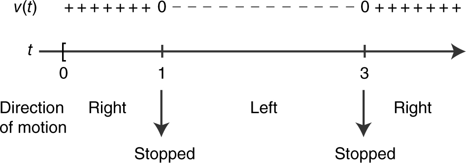
Figure 10.3-3

Step 4: Determine acceleration. (See Figure 10.3-4 .)

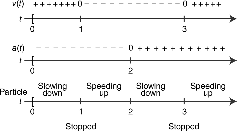
Figure 10.3-4

Step 5: Draw the motion of the particle. (See Figure 10.3-5 .) s (0) = –1, s (1) = 3, s (2) = 1 and s (3) = –1

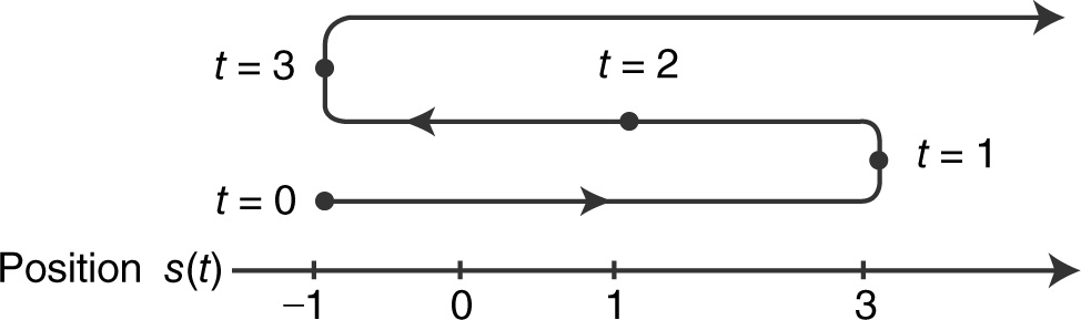
Figure 10.3-5

At t = 0, the particle is at –1 and moving to the right. It slows down and stops at t = 1 and at t = 3. It reverses direction (moving to the left) and speeds up until it reaches 1 at t = 2. It continues moving left but slows down and stops at –1 at t = 3. Then it reverses direction (moving to the right) again and speeds up indefinitely. (Note: “Speeding up” is defined as when |v (t )| increases and “slowing down” is defined as when |v (t )| decreases.)

10.4 Rapid Review

1. Write an equation of the normal line to the graph y = e^x at x = 0.

Answer :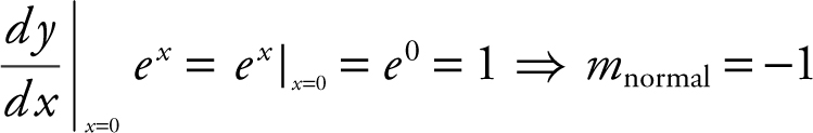
At x = 0, y = e ⁰ = 1 ⇒ you have the point (0, 1).
Equation of normal: y – 1 = –1(x – 0) or y = –x + 1.

2. Using your calculator, find the values of x at which the function y = –x ² + 3x and y = ln x have parallel tangents.

Answer :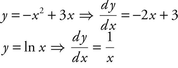
Set 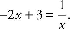Using the [Solve ] function on your calculator, enter
[Solve ] and obtain x = 1 or

3. Find the linear approximation of f (x ) = x ³ at x = 1 and use the equation to find f (1.1).

Answer : f (1) = 1 ⇒ (1, 1) is on the tangent line and f ′(x ) = 3x ² ⇒ f ′(1) = 3.
y – 1 = 3(x – 1) or y = 3x – 2.
f (1.1) ≈ 3(1.1) – 2 ≈ 1.3

4. (See Figure 10.4-1 .)
(a) When is the acceleration zero? (b) Is the particle moving to the right or left?

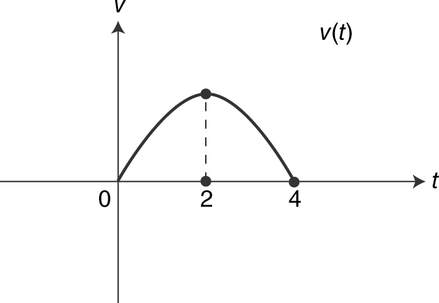
Figure 10.4-1

Answer : (a) a (t ) = v ′(t ) and v ′(t ) is the slope of the tangent. Thus, a (t ) = 0 at t = 2.

(b) Since v (t ) ≥ 0, the particle is moving to the right.

5. Find the maximum acceleration of the particle whose velocity function is v (t ) = t ² + 3 on the interval 0 ≤ t ≤ 4.

Answer : a (t ) = v ′(t ) = 2(t ) on the interval 0 ≤ t ≤ 4, a (t ) has its maximum value at t = 4. Thus a (t ) = 8. The maximum acceleration is 8.

10.5 Practice Problems

Part A—The use of a calculator is not allowed.

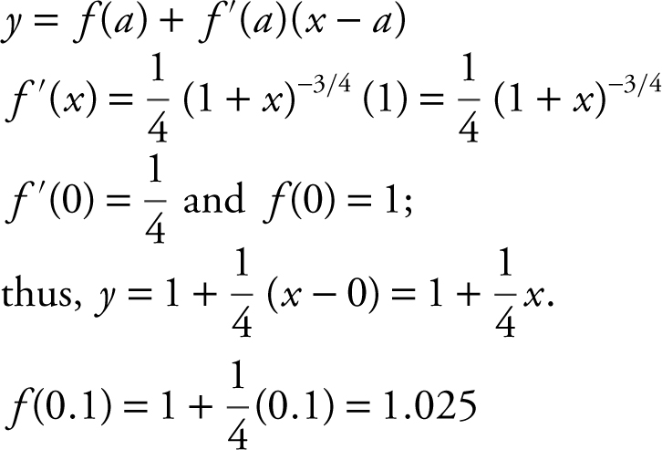
1 . Find the linear approximation of f (x ) = (1 + x )^1/4 at x = 0 and use the equation to approximate f (0.1).

2 . Find the approximate value of using linear approximation.

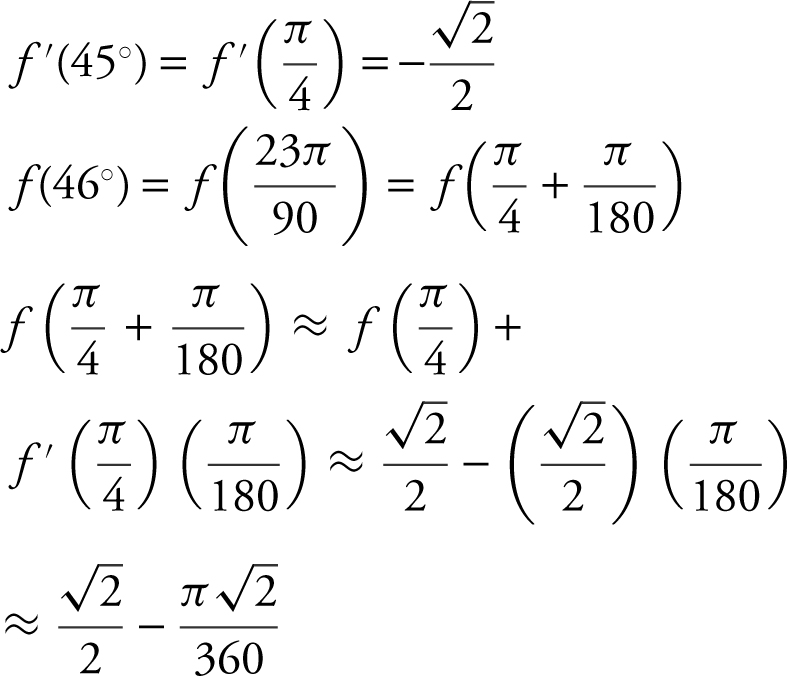
3 . Find the approximate value of cos 46° using linear approximation.

4 . Find the point on the graph of y = |x ³ | such that the tangent at the point is parallel to the line y – 12x = 3.

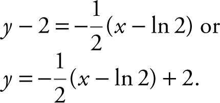
5 . Write an equation of the normal to the graph of y = e^x at x = ln 2.

6 . If the line y – 2x = b is tangent to the graph y = –x ² + 4, find the value of b .

7 . If the position function of a particle , find the velocity and position of particle when its acceleration is 0.

8 . The graph in Figure 10.5-1 represents the distance in feet covered by a moving particle in t seconds. Draw a sketch of the corresponding velocity function.

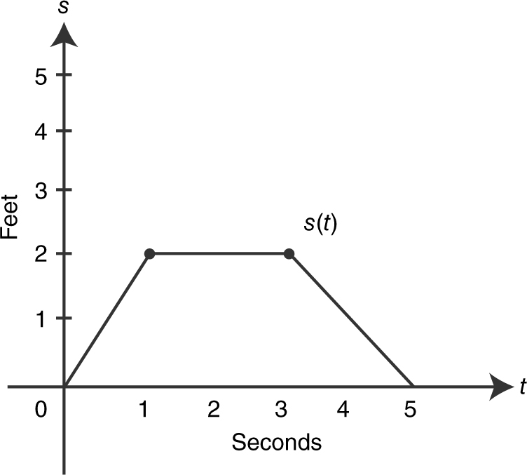
Figure 10.5-1

9 . The position function of a moving particle is shown in Figure 10.5-2 .

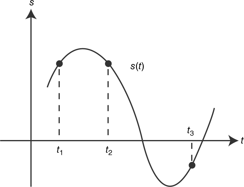
Figure 10.5-2

For which value(s) of t (t ₁ , t ₂ , t ₃ ) is:

(a) the particle moving to the left?

(b) the acceleration negative?

(c) the particle moving to the right and slowing down?

10 . The velocity function of a particle is shown in Figure 10.5-3 .

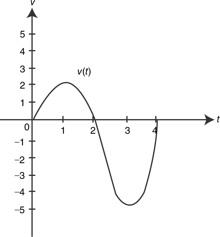
Figure 10.5-3

(a) When does the particle reverse direction?

(b) When is the acceleration 0?

(c) When is the speed the greatest?

11 . A ball is dropped from the top of a 640-foot building. The position function of the ball is s (t ) = –16t ² + 640, where t is measured in seconds and s (t ) is in feet. Find:

(a) The position of the ball after 4 seconds.

(b) The instantaneous velocity of the ball at t = 4.

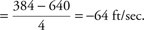
(c) The average velocity for the first 4 seconds.

(d) When the ball will hit the ground.

(e) The speed of the ball when it hits the ground.

12 . The graph of the position function of a moving particle is shown in Figure 10.5-4 .

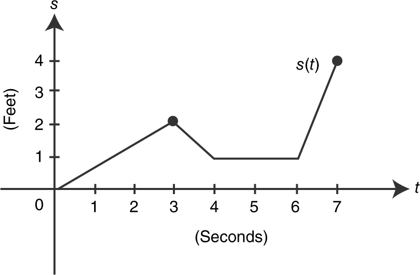
Figure 10.5-4

(a) What is the particle’s position at t = 5?

(b) When is the particle moving to the left?

(c) When is the particle standing still?

(d) When does the particle have the greatest speed?

Part B—Calculators are allowed.

13 . The position function of a particle moving on a line is s (t ) = t ³ – 3t ² + 1, t ≥ 0 where t is measured in seconds and s in meters. Describe the motion of the particle.

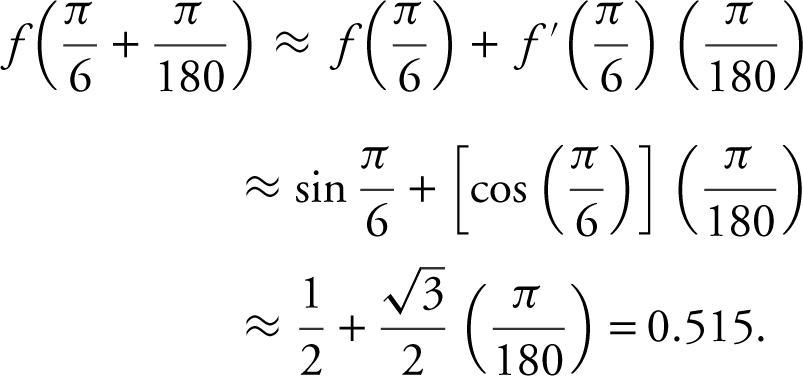
14 . Find the linear approximation of f (x ) = sin x at x = π . Use the equation to find the approximate value of .

15 . Find the linear approximation of f (x ) = ln (1 + x ) at x = 2.

16 . Find the coordinates of each point on the graph of y ² = 4 – 4x ² at which the tangent line is vertical. Write an equation of each vertical tangent.

17 . Find the value(s) of x at which the graphs of y = ln x and y = x ² + 3 have parallel tangents.

18 . The position functions of two moving particles are s ₁ (t ) = ln t and s ₂ (t ) = sin t and the domain of both functions is 1 ≤ t ≤ 8. Find the values of t such that the velocities of the two particles are the same.

19 . The position function of a moving particle on a line is s (t ) = sin(t ) for 0 ≤ t ≤ 2π . Describe the motion of the particle.

20 . A coin is dropped from the top of a tower and hits the ground 10.2 seconds later. The position function is given as s (t ) = –16t ² – v ₀ t + s ₀ , where s is measured in feet, t in seconds, and v ₀ is the initial velocity and s ₀ is the initial position. Find the approximate height of the building to the nearest foot.

10.6 Cumulative Review Problems

(Calculator) indicates that calculators are permitted.

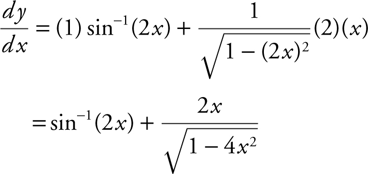
21 . Find if y = x sin^–1 (2x ).

22 . Given f (x ) = x ³ – 3x ² + 3x – 1 and the point (1, 2) is on the graph of f ^–1 (x ). Find the slope of the tangent line to the graph of f ^–1 (x ) at (1, 2).

23 . Evaluate .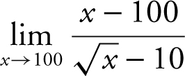

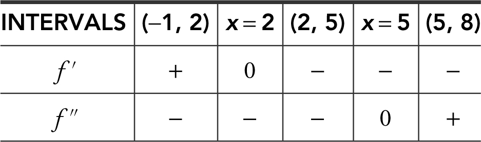
24 . A function f is continuous on the interval (–1, 8) with f (0) = 0, f (2) = 3, and f (8) = 1/2 and has the following properties:

(a) Find the intervals on which f is increasing or decreasing.

(b) Find where f has its absolute extrema.

(c) Find where f has the points of inflection.

(d) Find the intervals on which f is concave upward or downward.

(e) Sketch a possible graph of f .

25 . The graph of the velocity function of a moving particle for 0 ≤ t ≤ 8 is shown in Figure 10.6-1 . Using the graph:

(a) Estimate the acceleration when v (t ) = 3 ft/sec.

(b) Find the time when the acceleration is a minimum.

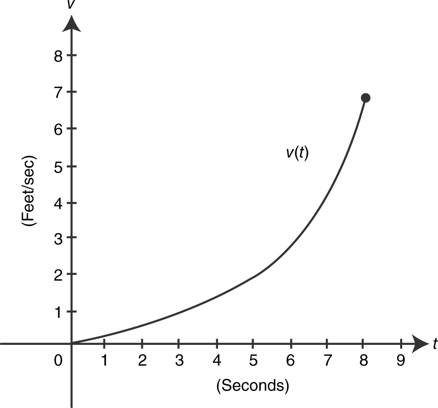
Figure 10.6-1

10.7 Solutions to Practice Problems

Part A—The use of a calculator is not allowed.

1 . Equation of tangent line:

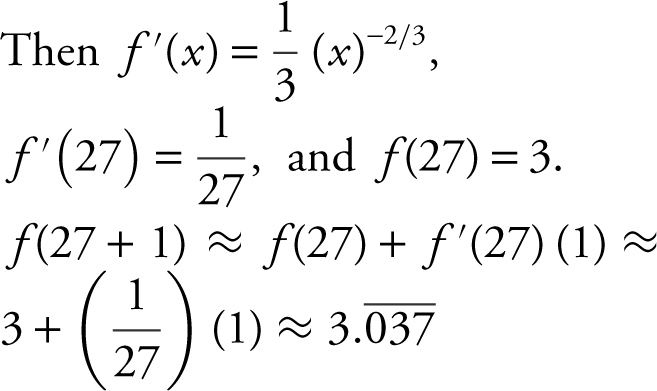
2 . f (a + Δx ) ≈ f (a ) + f ′(a )Δx

Let and f (28) = f (27+1).

3 . f (a + Δx ) ≈ f (a ) + f ′(a ) Δx Convert to radians:

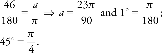
Let f (x ) = cos x and f (45°) =

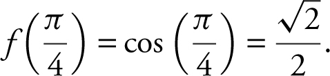
Then f ′(x ) = – sin x and

4 . Step 1: Find m _tangent .

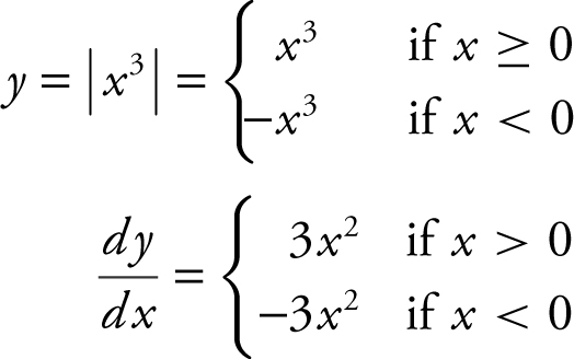
Step 2: Set m _tangent = slope of line y – 12x = 3.
Since y – 12x = 3 ⇒ y = 12x + 3, then m = 12.
Set 3x ² = 12 ⇒ x = ±2
since x ≥ 0, x = 2.
Set –3x ² = 12 ⇒ x ² = –4. Thus ∅.

Step 3: Find the point on the curve. (See Figure 10.7-1 .)

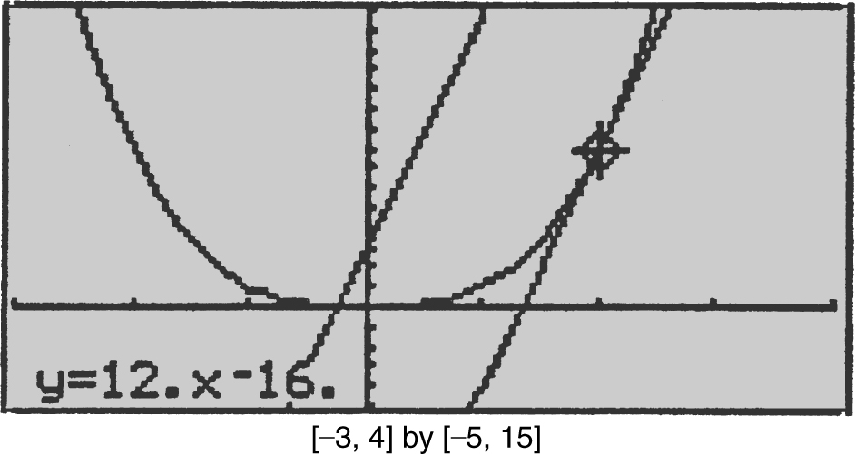
Figure 10.7-1

At x = 2, y = x ³ = 2³ = 8.
Thus, the point is (2, 8).

5 . Step 1: Find m _tangent .

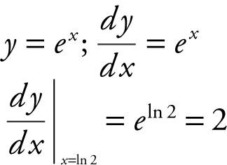
Step 2: Find m _normal .
At x = ln 2, m _normal =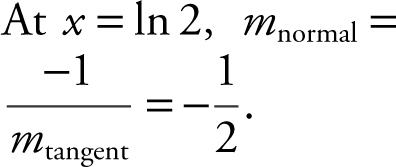

Step 3: Write equation of normal. At x = ln 2, y = e^x = e ^ln2 = 2. Thus the point of tangency is (ln 2, 2). The equation of normal:

6 . Step 1: Find m _tangent .

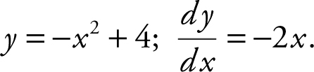
Step 2: Find the slope of line y – 2x = b
y – 2x = b ⇒
y = 2x + b or m = 2.

Step 3: Find point of tangency.

Set m _tangent = slope of line y – 2x = b ⇒ – 2x = 2 ⇒ x = –1.
At x = –1, y = –x ² + 4 = –(–1)² + 4 = 3; (–1, 3).

Step 4: Find b .

Since the line y – 2x = b passes through the point (–1, 3), thus 3 – 2(–1) = b or b = 5.

7 . v (t ) = s ′(t ) = t ² – 6t ;
a (t ) = v ′(t ) = s ″(t ) = 2t – 6
Set a (t ) = 0 ⇒ 2t – 6 = 0 or t = 3. v (3) = (3)² – 6(3) = – 9;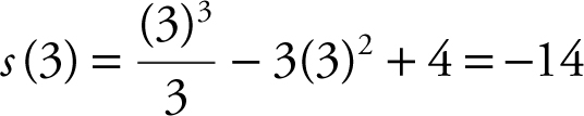
.

8 . On the interval (0, 1), the slope of the line segment is 2. Thus the velocity v (t ) = 2 ft/sec. On (1, 3), v (t ) = 0 and on (3, 5), v (t ) = –1. (See Figure 10.7-2 .)

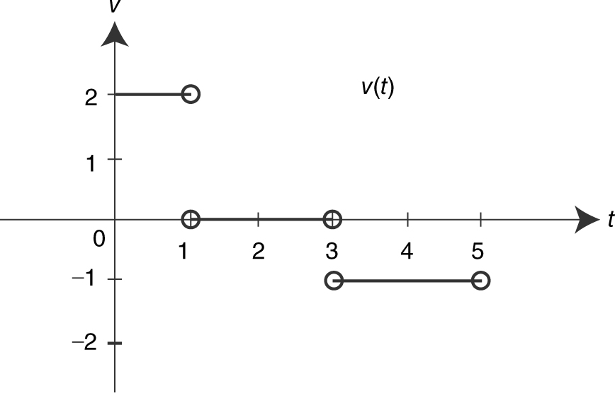
Figure 10.7-2

9 . (a) At t = t ₂ , the slope of the tangent is negative. Thus, the particle is moving to the left.

(b) At t = t ₁ , and at t = t ₂ , the curve is concave downward acceleration is negative.

(c) At t = t ₁ , the slope > 0 and thus the particle is moving to the right. The curve is concave downward ⇒ the particle is slowing down.

10 . (a) At t = 2, v (t ) changes from positive to negative, and thus the particle reverses its direction.

(b) At t = 1, and at t = 3, the slope of the tangent to the curve is 0. Thus, the acceleration is 0.

(c) At t = 3, speed is equal to |– 5| = 5 and 5 is the greatest speed.

11 . (a) s (4) = –16(4)² + 640 = 384 ft

(b) v (t ) = s ′(t ) = –32t
v (4) =–32(4) ft/s = –128 ft/sec

(c) Average velocity =

(d) Set s (t ) = 0 ⇒ –16t ² + 640 = 0 ⇒ 16t ² = 640 or t = ± .
Since t ≥ 0, or t = ± or t ≈ 6.32 sec.

(e) |v ( )| = |–32( | = | – 64 | ft/s or ≈ 202.39 ft/sec

12 . (a) At t = 5, s (t ) = 1.

(b) For 3 < t < 4, s (t ) decreases. Thus, the particle moves to the left when 3 < t < 4.

(c) When 4 < t < 6, the particle stays at 1.

(d) When 6 < t < 7, speed = 2 ft/sec, the greatest speed, which occurs where s has the greatest slope.

Part B—Calculators are allowed.

13 . Step 1: v (t ) = 3t ² – 6t
a (t ) = 6t – 6

Step 2: Set v (t ) = 0 ⇒ 3t ² – 6t = 0 ⇒ 3t (t – 2) = 0, or t = 0 or t = 2 Set a (t ) = 0 ⇒ 6t – 6 = 0 or t = 1.

Step 3: Determine the directions of motion. (See Figure 10.7-3 .)

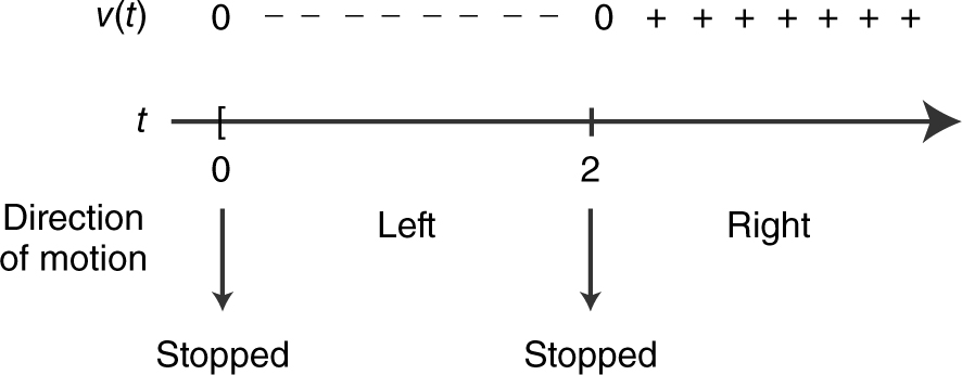
Figure 10.7-3

Step 4: Determine acceleration. (See Figure 10.7-4 .)

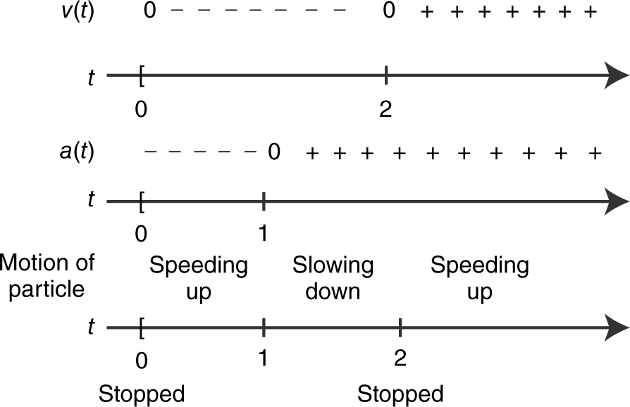
Figure 10.7-4

Step 5: Draw the motion of the particle. (See Figure 10.7-5 .) s (0) = 1, s (1) = –1, and s (2) = –3.

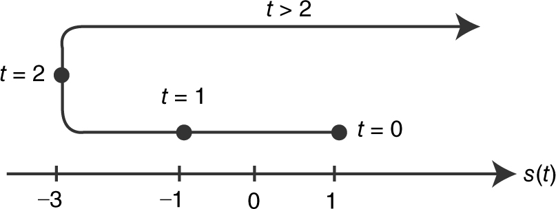
Figure 10.7-5

The particle is initially at 1 (t = 0). It moves to the left speeding up until t = 1, when it reaches –1. Then it continues moving to the left, but slowing down until t = 2 at –3. The particle reverses direction, moving to the right and speeding up indefinitely.

14 . Linear approximation:
y = f (a ) + f ′(a )(x – a ) a = π
f (x ) = sin x and f (π ) = sin π = 0
f ′(x ) = cos x and f ′(π ) = cos π = –1.
Thus, y = 0 + (–1)(x –π ) or
y = –x + π .
is approximately:
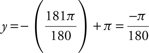or ≈ –0.0175.

15 . y = f (a ) + f ′(a )(x – a )
f (x ) = ln (1 + x ) and f (2) = ln (1 + 2) = ln 3

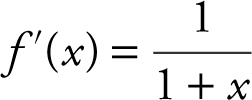and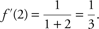

Thus, .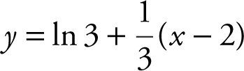

16 . Step 1: Find .
y ² = 4 – 4x ²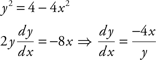

Step 2: Find .

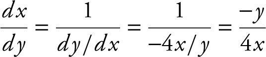
Set 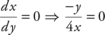or y = 0.

Step 3: Find points of tangency.

At y = 0, y ² = 4 – 4x ² becomes 0 = 4 – 4x ²
⇒ x = ±1.
Thus, points of tangency are (1, 0) and (–1, 0).

Step 4: Write equations of vertical tangents x = 1 and x = –1.

17 . Step 1: Find for y = ln x and y = x² + 3.

Step 2: Find the x -coordinate of point(s) of tangency.
Parallel tangents ⇒ slopes are equal. Set .
Using the [Solve ] function of your calculator, enter [Solve ] and obtain or . Since for y = ln x , .

18 . s ₁ (t ) = ln t and .

s ₂ (t ) = sin(t ) and
s ′₂ (t ) = cos(t ); 1 ≤ t ≤ 8.

Enter and y ² = cos(x ). Use the [Intersection ] function of the calculator and obtain t = 4.917 and t = 7.724.

19 . Step 1: s (t ) = sin t
v (t ) = cos t
a (t ) = – sin t

Step 2: Set v (t ) = 0 ⇒ cos t = 0;
and .
Set a (t ) = 0 ⇒ – sin t = 0; t =π and 2π.

Step 3: Determine the directions of motion. (See Figure 10.7-6 .)

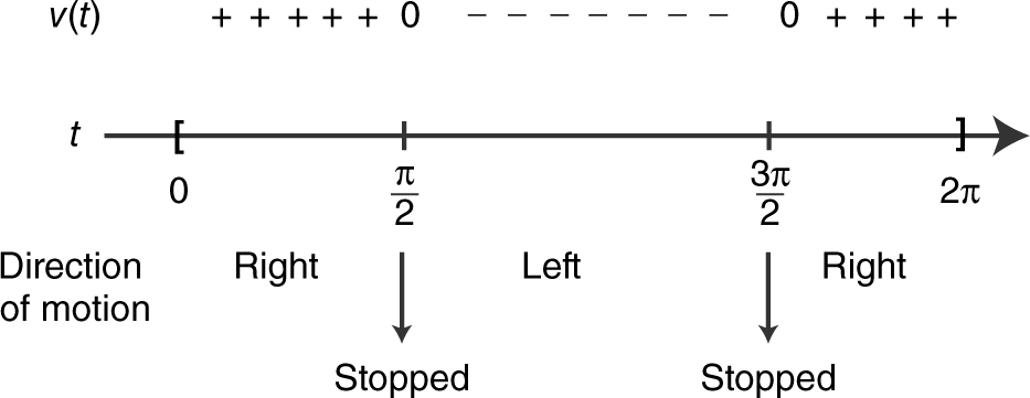
Figure 10.7-6

Step 4: Determine acceleration. (See Figure 10.7-7 .)

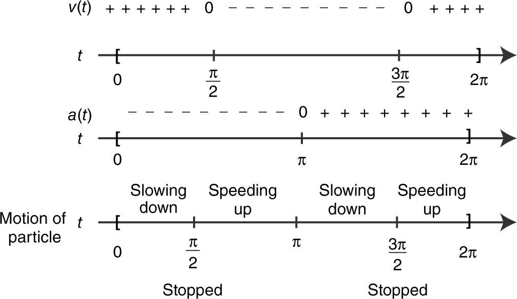
Figure 10.7-7

Step 5: Draw the motion of the particle. (See Figure 10.7-8 .)

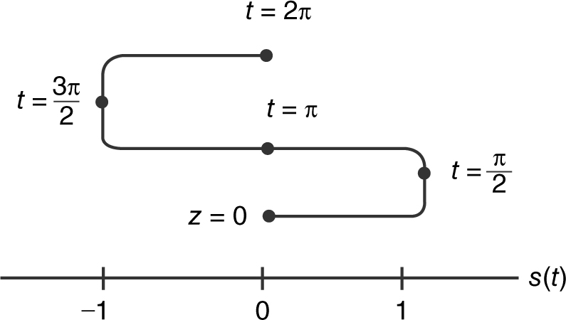
Figure 10.7-8

The particle is initially at 0, s (0) = 0. It moves to the right but slows down to a stop at 1 when = 1. It then turns and moves to the left speeding up until it reaches 0, when t = π, s (π) = 0 and continues to the left, but slowing down to a stop at – 1 when . It then turns around again, moving to the right, speeding up to 0 when t = 2π, s (2π) = 0.

20 . s (t ) = – 16t ² + v ₀ t + s ₀
s ₀ = height of building and v ₀ = 0.
Thus, s (t ) =– 16t ² + s ₀ .
When the coin hits the ground, s (t ) = 0, t = 10.2. Thus, set s (t ) = 0 ⇒ – 16t ² + s ₀ = 0 ⇒ – 16(10.2)² + s ₀ = 0 s ₀ = 1664.64 ft. The building is approximately 1665 ft tall.

10.8 Solutions to Cumulative Review Problems

21 . Using product rule, let u = x ; v = sin^–1 (2x ).

22 . Let y = f (x ) ⇒ y = x ³ – 3x ² + 3x – 1. To find f ^–1 (x ), switch x and
y : x = y ³ – 3y ² + 3y – 1.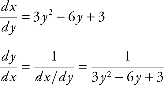

23 . Substituting x = 100 into the expression 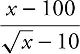would lead to . Apply L’Hôpital’s Rule, and you have 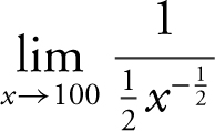or 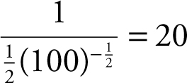. Another approach to solve the problem is as follows. Multiply both numerator and denominator by the conjugate of the denominator ( + 10):

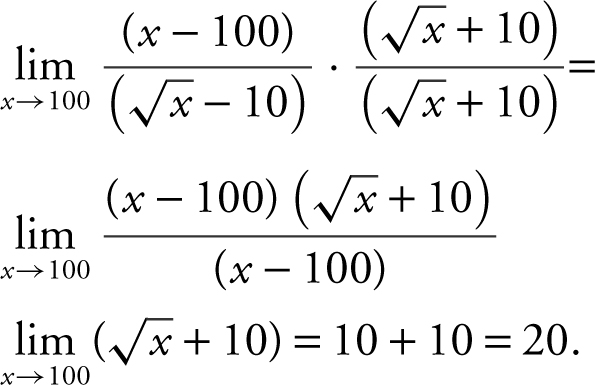
An alternative solution is to factor the numerator: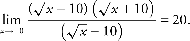

24 . (a) f ′ > 0 on (–1, 2), f is increasing on (–1, 2), f ′< 0 on (2, 8), f is decreasing on (2, 8).

(b) At x = 2, f ′ = 0 and f ″ < 0, thus at x = 2, f has a relative maximum. Since it is the only relative extremum on the interval, it is an absolute maximum. Since f is a continuous function on a closed interval and at its endpoints f(–1) < 0 and f (8) = 1/2, f has an absolute minimum at x = –1.

(c) At x = 5, f has a change of concavity and f ′ exists at x = 5.

(d) f ″ < 0 on (–1, 5), f is concave downward on (–1, 5).
f ″ > 0 on (5, 8), f is concave upward on (5, 8).

(e) A possible graph of f is given in Figure 10.8-1 .

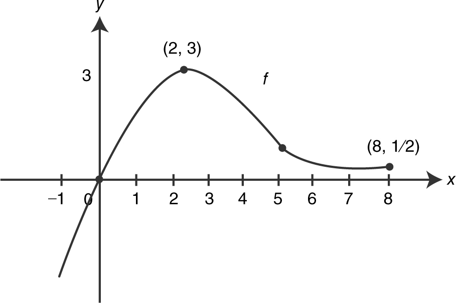
Figure 10.8-1

25 . (a) v (t ) = 3 ft/sec at t = 6. The tangent line to the graph of v (t ) at t = 6 has a slope of approximately m = 1. (The tangent passes through the points (8, 5) and (6, 3); thus m = 1.) Therefore the acceleration is 1 ft/sec² .

(b) The acceleration is a minimum at t = 0, since the slope of the tangent to the curve of v (t ) is the smallest at t = 0.