5 Steps to a 5: AP Calculus AB 2017 (2016)

STEP 4

Review the Knowledge You Need to Score High

CHAPTER 6

Big Idea 1: Limits

Limits and Continuity

IN THIS CHAPTER

Summary: On the AP Calculus AB exam, you will be tested on your ability to find the limit of a function. In this chapter, you will be shown how to solve several types of limit problems which include finding the limit of a function as x approaches a specific value, finding the limit of a function as xapproaches infinity, one-sided limits, infinite limits, and limits involving sine and cosine. You will also learn how to apply the concepts of limits to finding vertical and horizontal asymptotes as well as determining the continuity of a function.

Key Ideas

Definition of the limit of a function

Properties of limits

Evaluating limits as x approaches a specific value

Evaluating limits as x approaches ± infinity

One-sided limits

Limits involving infinities

Limits involving sine and cosine

Vertical and horizontal asymptotes

Continuity

6.1 The Limit of a Function

Main Concepts: Definition and Properties of Limits, Evaluating Limits, One-Sided Limits, Squeeze Theorem

Definition and Properties of Limits

Definition of Limit

Let f be a function defined on an open interval containing a , except possibly at a itself. Then (read as the limit of f (x ) as x approaches a is L ) if for any ε > 0, there exists a δ > 0 such that | f (x ) – L | < ε whenever |x– a | < δ .

Properties of Limits

Given and and L , M , a , c , and n are real numbers, then:

1.

2.

3.

4.

5.

6.

Evaluating Limits

If f is a continuous function on an open interval containing the number a , then = f (a ).

Common techniques in evaluating limits are:

1. Substituting directly

2. Factoring and simplifying

3. Multiplying the numerator and denominator of a rational function by the conjugate of either the numerator or denominator

4. Using a graph or a table of values of the given function

Example 1

Find the limit: .

Substituting directly: .

Example 2

Find the limit: .

Using the product rule, .

Example 3

Find the limit: .

Factoring and simplifying: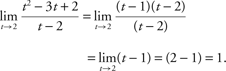

(Note that had you substituted t = 2 directly in the original expression, you would have obtained a zero in both the numerator and denominator.)

Example 4

Find the limit: .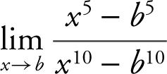

Factoring and simplifying: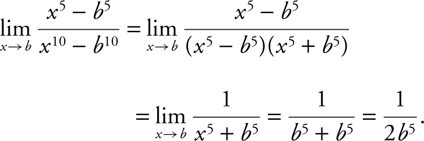

Example 5

Find the limit: .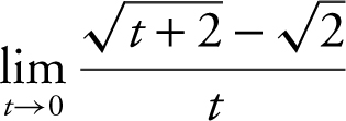

Multiplying both the numerator and the denominator by the conjugate of the numerator,

(Note that substituting 0 directly into the original expression would have produced a 0 in both the numerator and denominator.)

Example 6

Find the limit: .

Enter in the calculator. You see that the graph of f (x ) approaches 3 as x approaches 0. Thus, the . (Note that had you substituted x = 0 directly in the original expression, you would have obtained a zero in both the numerator and denominator.) (See Figure 6.1-1 .)

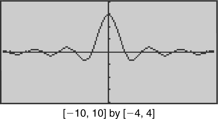
Figure 6.1-1

Example 7

Find the limit: .

Enter into your calculator. You notice that as x approaches 3 from the right, the graph of f (x ) goes higher and higher, and that as x approaches 3 from the left, the graph of f (x ) goes lower and lower. Therefore, is undefined. (See Figure 6.1-2 .)

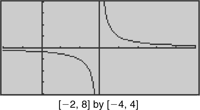
Figure 6.1-2

• Always indicate what the final answer is, e.g., “The maximum value of f is 5.” Use complete sentences whenever possible.

One-Sided Limits

Let f be a function and let a be a real number. Then the right-hand limit: represents the limit of f as x approaches a from the right, and the left-hand limit: represents the limit of f as x approaches a from the left.

Existence of a Limit

Let f be a function and let a and L be real numbers. Then the two-sided limit: if and only if the one-sided limits exist and .

Example 1

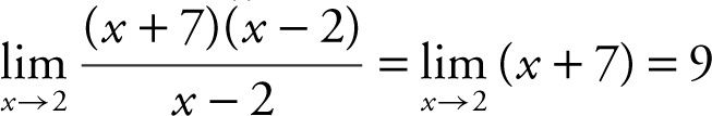
Given , find the limits: (a) , (b) , and (c) . Substituting x = 3 into f (x ) leads to a 0 in both the numerator and denominator. Factor f (x ) as which is equivalent to (x + 1) where x ≠ 3. Thus, (a) , (b) , and (c) since the one-sided limits exist and are equal, , therefore the two-sided limit exists and 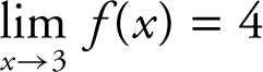. (Note that f (x ) is undefined at x = 3, but the function gets arbitrarily close to 4 as x approaches 3. Therefore the limit exists.) (See Figure 6.1-3 .)

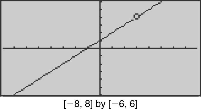
Figure 6.1-3

Example 2

Given f (x ) as illustrated in the accompanying diagram (Figure 6.1-4 ), find the limits: (a) , (b) , and (c) .

Figure 6.1-4

(a) As x approaches 0 from the left, f (x ) gets arbitrarily close to 0. Thus, = 0.

(b) As x approaches 0 from the right, f (x ) gets arbitrarily close to 2. Therefore, = 2. Note that f (0) ≠ 2.

(c) Since 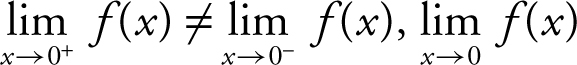does not exist.

Example 3

Given the greatest integer function f (x ) = [x ], find the limits: (a) , (b) , and (c) .

(a) Enter y 1 = int(x ) in your calculator. You see that as x approaches 1 from the right, the function stays at 1. Thus, . Note that f (1) is also equal to 1.

(b) As x approaches 1 from the left, the function stays at 0. Therefore, . Notice that .

(c). Since , therefore, 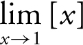does not exist. (See Figure 6.1-5 .)

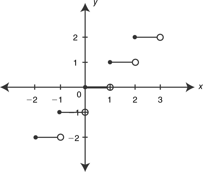
Figure 6.1-5

Example 4

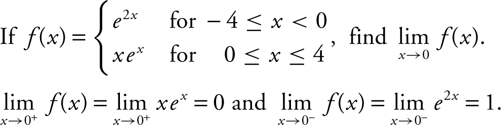
Given 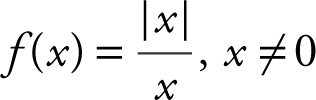, find the limits: (a) , (b) , and (c) . (a) From inspecting the graph, , (b) , and (c) since , therefore, does not exist. (See Figure 6.1-6 .)

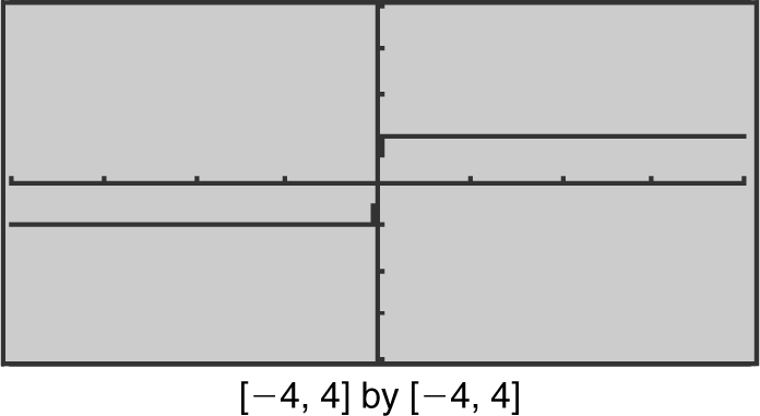
Figure 6.1-6

Example 5

Thus, does not exist.

• Remember ln(e ) = 1 and e ^ln3 = 3 since y = ln x and y = e ^x are inverse functions.

Squeeze Theorem

If f , g , and h are functions defined on some open interval containing a such that g (x ) ≤ f (x ) ≤ h (x ) for all x in the interval except possibly at a itself, and , then .

Theorems on Limits

(1) and (2)

Example 1

Find the limit if it exists: .

Substituting 0 into the expression would lead to 0/0. Rewrite as and thus, 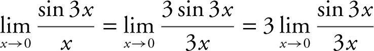. As x approaches 0, so does 3x . Therefore, 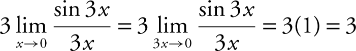. (Note that is equivalent to by replacing 3x by x .) Verify your result with a calculator. (See Figure 6.1-7 .)

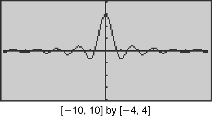
Figure 6.1-7

Example 2

Find the limit if it exists: .

Rewrite as 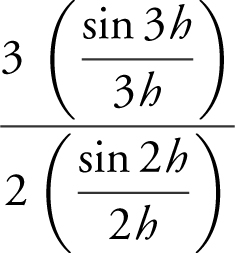. As h approaches 0, so do 3h and 2h . Therefore,

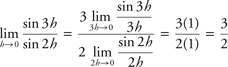. (Note that substituting h = 0 into the original expression would have produced 0/0.) Verify your result with a calculator. (See Figure 6.1-8 .)

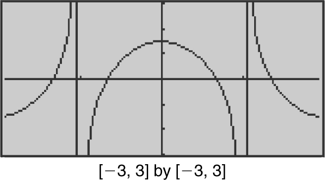
Figure 6.1-8

Example 3

Find the limit if it exists: .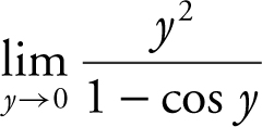

Substituting 0 in the expression would lead to 0/0. Multiplying both the numerator and denominator by the conjugate (1 + cos y ) produces . = (1)² (1 + 1) = 2. (Note that 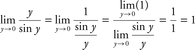.) Verify your result with a calculator. (See Figure 6.1-9 .)

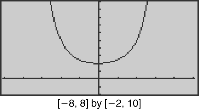
Figure 6.1-9

Example 4

Find the limit if it exists: .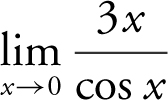

Using the quotient rule for limits, you have 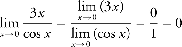. Verify your result with a calculator. (See Figure 6.1-10 .)

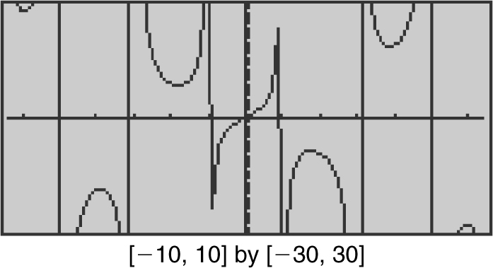
Figure 6.1-10

6.2 Limits Involving Infinities

Main Concepts: Infinite Limits (as x → a ), Limits at Infinity (as x → ∞), Horizontal and Vertical Asymptotes

Infinite Limits (as x → a )

If f is a function defined at every number in some open interval containing a , except possibly at a itself, then

(1) 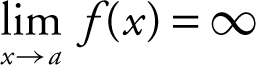means that f (x ) increases without bound as x approaches a .

(2) 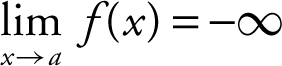means that f (x ) decreases without bound as x approaches a .

Limit Theorems

(1) If n is a positive integer, then

(a)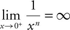

(b)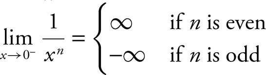

(2) If the 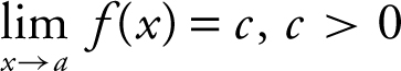, and 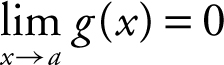, then

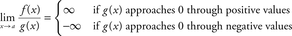
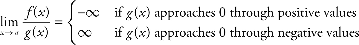
(3) If the 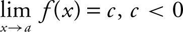, and , then

(Note that limit theorems 2 and 3 hold true for x → a ⁺ and x → a ^– .)

Example 1

Evaluate the limit: (a) and (b) .

(a) The limit of the numerator is 5 and the limit of the denominator is 0 through positive values. Thus, . (b) The limit of the numerator is 5 and the limit of the denominator is 0 through negative values. Therefore, . Verify your result with a calculator. (See Figure 6.2-1 .)

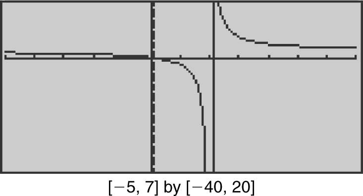
Figure 6.2-1

Example 2

Find: .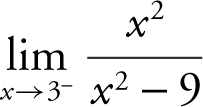

Factor the denominator obtaining 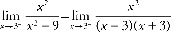. The limit of the numerator is 9 and the limit of the denominator is (0)(6) = 0 through negative values. Therefore, 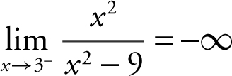. Verify your result with a calculator. (See Figure 6.2-2 .)

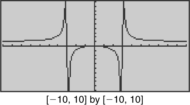
Figure 6.2-2

Example 3

Find: .

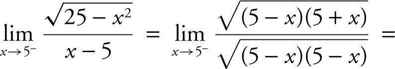
Substituting 5 into the expression leads to 0/0. Factor the numerator into . As x → 5^– , (x – 5) < 0. Rewrite (x – 5) as –(5 – x ) as x → 5^– , (5 – x ) > 0 and thus, you may express (5 – x ) as . Therefore, . Substituting these equivalent expressions into the original problem, you have 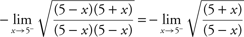. The limit of the numerator is 10 and the limit of the denominator is 0 through positive values. Thus, the .

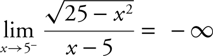Example 4

Find: 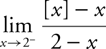, where [x ] is the greatest integer value of x .

As x → 2^– , [x ] = 1. The limit of the numerator is (1 – 2) = –1. As x → 2^– , (2 – x ) = 0 through positive values. Thus, .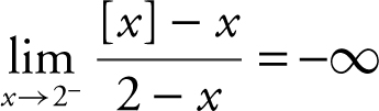

• Do easy questions first. The easy ones are worth the same number of points as the hard ones.

Limits at Infinity (as x → ± ∞)

If f is a function defined at every number in some interval (a , ∞), then means that L is the limit of f (x ) as x increases without bound. If f is a function defined at every number in some interval (–∞, a ), then means that L is the limit of f (x ) as x decreases without bound.

Limit Theorem

If n is a positive integer, then

(a)

(b)

Example 1

Evaluate the limit: .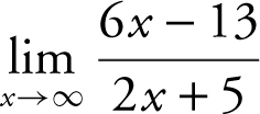

Divide every term in the numerator and denominator by the highest power of x (in this case, it is x ), and obtain:

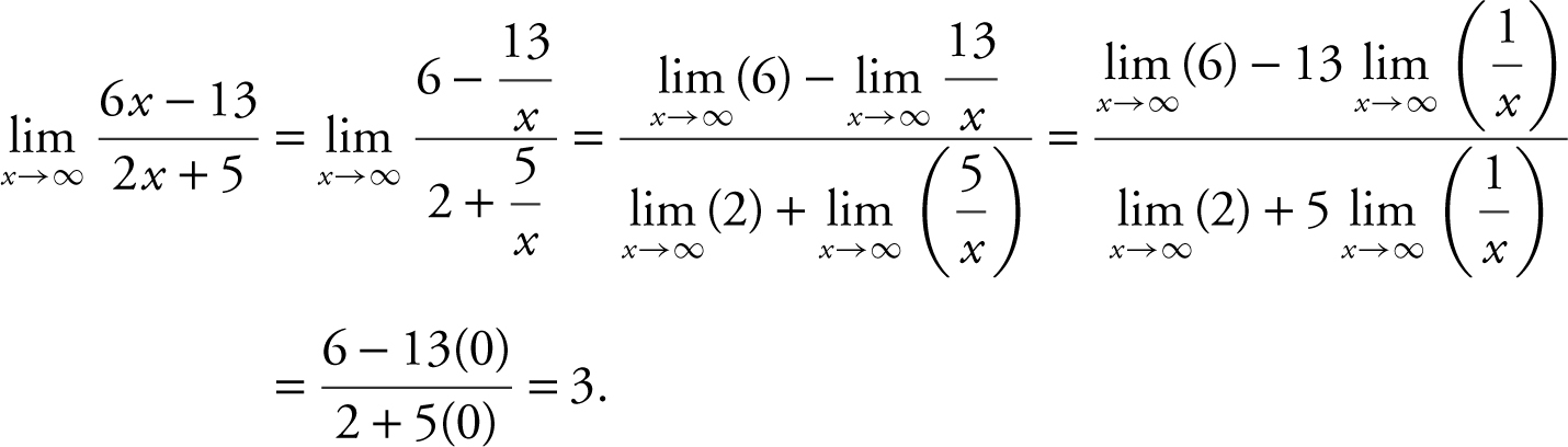
Verify your result with a calculator. (See Figure 6.2-3 .)

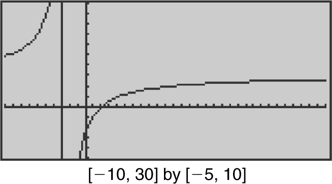
Figure 6.2-3

Example 2

Evaluate the limit: .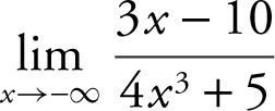

Divide every term in the numerator and denominator by the highest power of x . In this case, it is x ³ . Thus,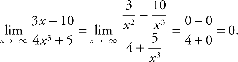

Verify your result with a calculator. (See Figure 6.2-4 .)

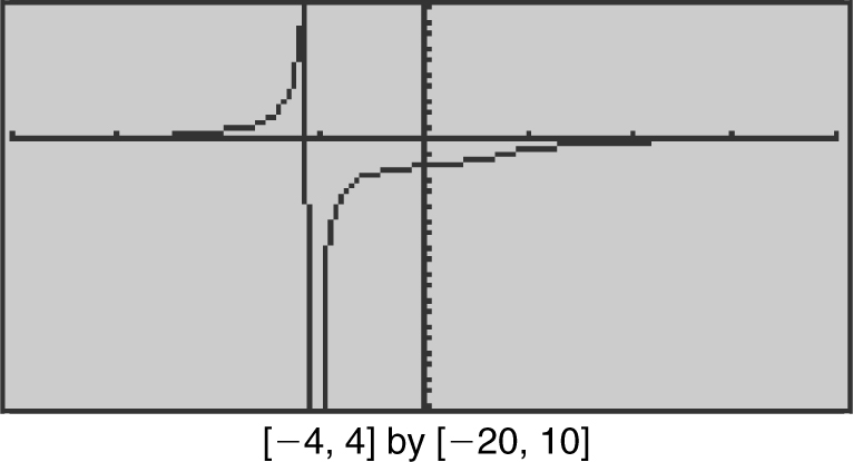
Figure 6.2-4

Example 3

Evaluate the limit: .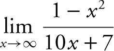

Divide every term in the numerator and denominator by the highest power of x . In this case, it is x ² . Therefore, 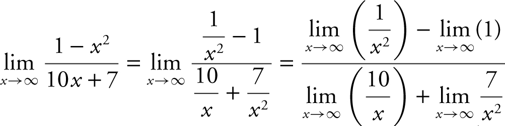. The limit of the numerator is –1 and the limit of the denominator is 0. Thus, .

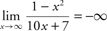Verify your result with a calculator. (See Figure 6.2-5 .)

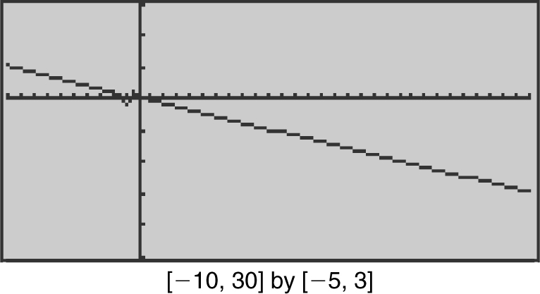
Figure 6.2-5

Example 4

Evaluate the limit: .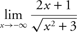

As x → –∞, x < 0 and thus, . Divide the numerator and denominator by x (not x ² since the denominator has a square root). Thus, you have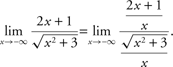

Replacing the x below by , you have

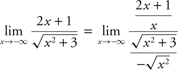
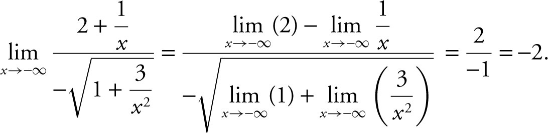
Verify your result with a calculator. (See Figure 6.2-6 .)

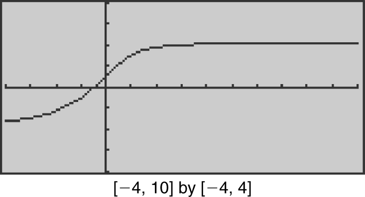
Figure 6.2-6

• Remember that ln = ln (1) – ln x = – ln x and y = e ^–x .

Horizontal and Vertical Asymptotes

A line y = b is called a horizontal asymptote for the graph of a function f if either = b or = b .

A line x = a is called a vertical asymptote for the graph of a function f if either = +∞ or = +∞.

Example 1

Find the horizontal and vertical asymptotes of the function .

To find the horizontal asymptotes, examine the and the .

The 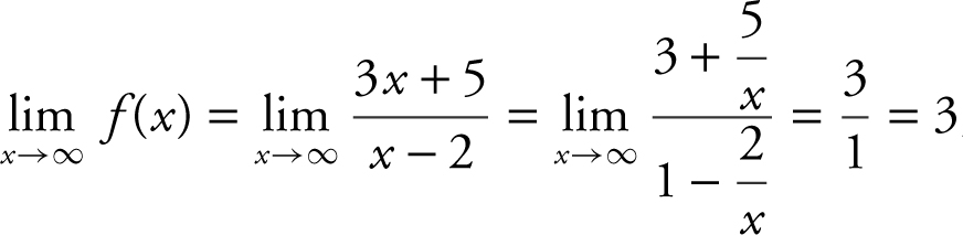, and the .

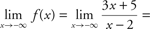
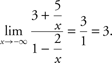Thus, y = 3 is a horizontal asymptote.

To find the vertical asymptotes, look for x values such that the denominator (x – 2) would be 0, in this case, x = 2. Then examine:

(a) 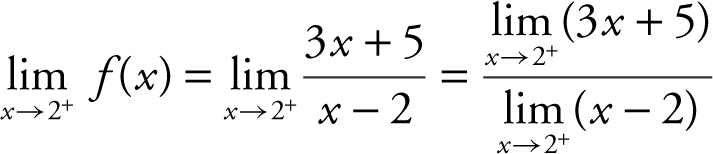, the limit of the numerator is 11 and the limit of the denominator is 0 through positive values, and thus, .

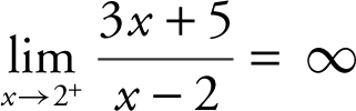(b) , the limit of the numerator is 11 and the limit of the denominator is 0 through negative values, and thus, .

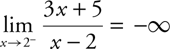Therefore, x = 2 is a vertical asymptote.

Example 2

Using your calculator, find the horizontal and vertical asymptotes of the function f (x ) = .

Enter . The graph shows that as x → ±∞, the function approaches 0, thus . Therefore, a horizontal asymptote is y = 0 (or the x -axis).

For vertical asymptotes, you notice that , and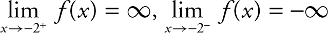 . Thus, the vertical asymptotes are x = –2 and x = 2. (See Figure 6.2-7 .)

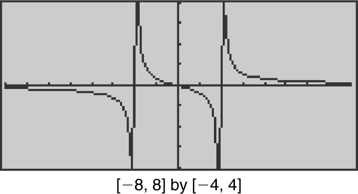
Figure 6.2-7

Example 3

Using your calculator, find the horizontal and vertical asymptotes of the function f (x ) = .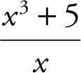

Enter 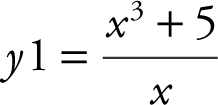. The graph of f (x ) shows that as x increases in the first quadrant, f (x ) goes higher and higher without bound. As x moves to the left in the second quadrant, f (x ) again goes higher and higher without bound. Thus, you may conclude that and and thus, f (x ) has no horizontal asymptote. For vertical asymptotes, you notice that , and . Therefore, the line x = 0 (or the y -axis) is a vertical asymptote. (See Figure 6.2-8 .)

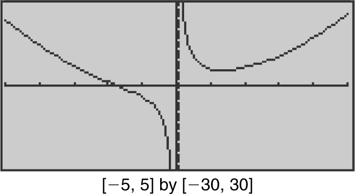
Figure 6.2-8

Relationship between the limits of rational functions as x → ∞ and horizontal asymptotes:

Given , then:

(1) If the degree of p (x ) is the same as the degree of q (x ), then , where a is the coefficient of the highest power of x in p (x ) and b is the coefficient of the highest power of x in q (x ). The line is a horizontal asymptote. See Example 1 on page 96 .

(2) If the degree of p (x ) is smaller than the degree of q (x ), then . The line y = 0 (or x -axis) is a horizontal asymptote. See Example 2 on page 97 .

(3) If the degree of p (x ) is greater than the degree of q (x ), then and . Thus, f (x ) has no horizontal asymptote. See Example 3 on page 97 .

Example 4

Using your calculator, find the horizontal asymptotes of the function .

Enter . The graph shows that f (x ) oscillates back and forth about the x -axis. As x → ±∞, the graph gets closer and closer to the x -axis which implies that f (x ) approaches 0. Thus, the line y = 0 (or the x -axis) is a horizontal asymptote. (See Figure 6.2-9 .)

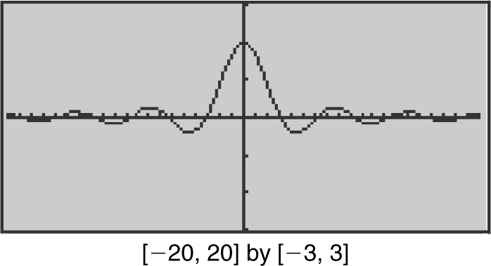
Figure 6.2-9

• When entering a rational function into a calculator, use parentheses for both the numerator and denominator, e.g., (x – 2) + (x + 3).

6.3 Continuity of a Function

Main Concepts: Continuity of a Function at a Number, Continuity of a Function over an Interval, Theorems on Continuity

Continuity of a Function at a Number

A function f is said to be continuous at a number a if the following three conditions are satisfied:

1. f (a ) exists

2.

3.

The function f is said to be discontinuous at a if one or more of these three conditions are not satisfied and a is called the point of discontinuity.

Continuity of a Function over an Interval

A function is continuous over an interval if it is continuous at every point in the interval.

Theorems on Continuity

1. If the functions f and g are continuous at a , then the functions f + g , f – g , f · g , f /g , and g (a ) ≠ 0, are also continuous at a .

2. A polynomial function is continuous everywhere.

3. A rational function is continuous everywhere, except at points where the denominator is zero.

4. Intermediate Value Theorem: If a function f is continuous on a closed interval [a , b ] and k is a number with f (a ) ≤ k ≤ f (b ), then there exists a number c in [a , b ] such that f (c ) = k .

Example 1

Find the points of discontinuity of the function .

Since f (x ) is a rational function, it is continuous everywhere, except at points where the denominator is 0. Factor the denominator and set it equal to 0: (x – 2)(x + 1) = 0. Thus x = 2 or x = –1. The function f (x ) is undefined at x = –1 and at x = 2. Therefore, f (x ) is discontinuous at these points. Verify your result with a calculator. (See Figure 6.3-1 .)

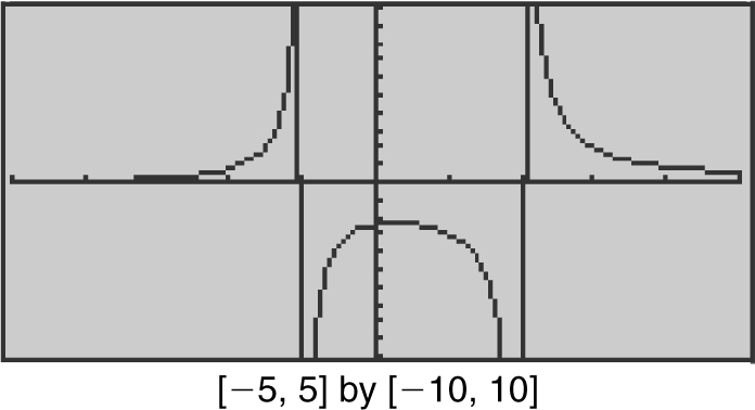
Figure 6.3-1

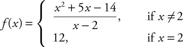
Example 2

Determine the intervals on which the given function is continuous:

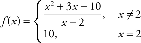
Check the three conditions of continuity at x = 2:

Condition 1: f (2) = 10.

Condition 2: .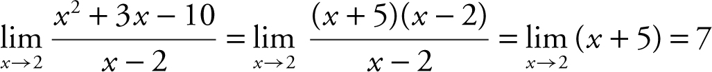

Condition 3: 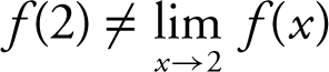. Thus, f (x ) is discontinuous at x = 2.

The function is continuous on (–∞, 2) and (2, ∞). Verify your result with a calculator. (See Figure 6.3-2 .)

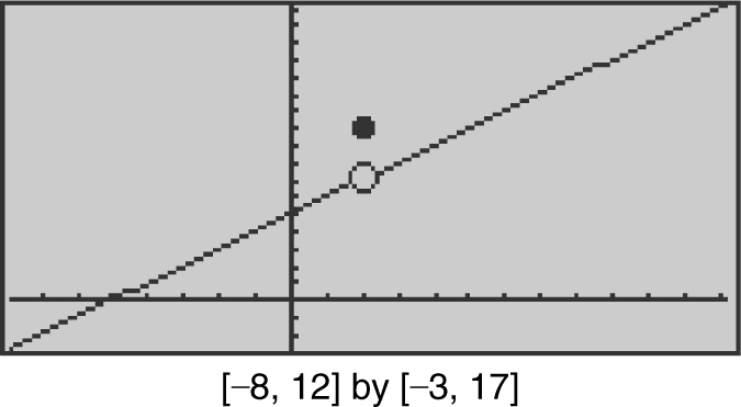
Figure 6.3-2

• Remember that and .

Example 3

For what value of k is the function 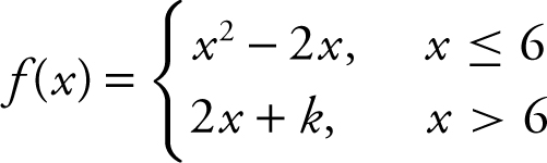continuous at x = 6?

For f (x ) to be continuous at x = 6, it must satisfy the three conditions of continuity:

Condition 1: f (6) = 6² – 2(6) = 24.

Condition 2: 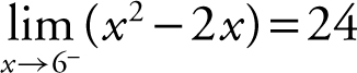; thus must also be 24 in order for the to equal 24. Thus, which implies 2(6) + k = 24 and k = 12. Therefore, if k = 12,

Condition (3): is also satisfied.

Example 4

Given f (x ) as shown in Figure 6.3-3 , (a) find f (3) and , and (b) determine if f (x ) is continuous at x = 3? Explain your answer.

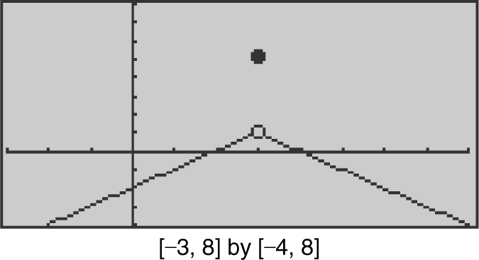
Figure 6.3-3

(a) The graph of f (x ) shows that f (3) = 5 and the 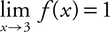. (b) Since , f (x ) is discontinuous at x = 3.

Example 5

If g (x ) = x ² – 2x – 15, using the Intermediate Value Theorem show that g (x ) has a root in the interval [1, 7].

Begin by finding g (1) and g (7), and g (1) = –16 and g (7) = 20. If g (x ) has a root, then g (x ) crosses the x -axis, i.e., g (x ) = 0. Since –16 ≤ 0 ≤ 20, by the Intermediate Value Theorem, there exists at least one number c in [1, 7] such that g (c ) = 0. The number c is a root of g (x ).

Example 6

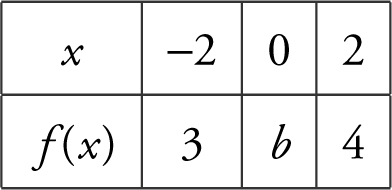
A function f is continuous on [0, 5], and some of the values of f are shown below.

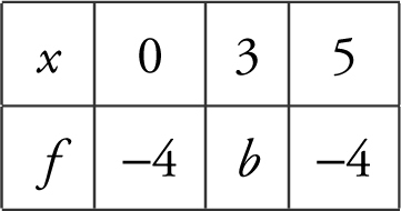
If f (x ) = –2 has no solution on [0, 5], then b could be

(A) 1

(B) 0

(C) –2

(D) –5

If b = –2, then x = 3 would be a solution for f (x ) = –2.

If b = 0, 1, or 3, f (x ) = –2 would have two solutions for f (x ) = –2.

Thus, b = –5, choice (D). (See Figure 6.3-4 .)

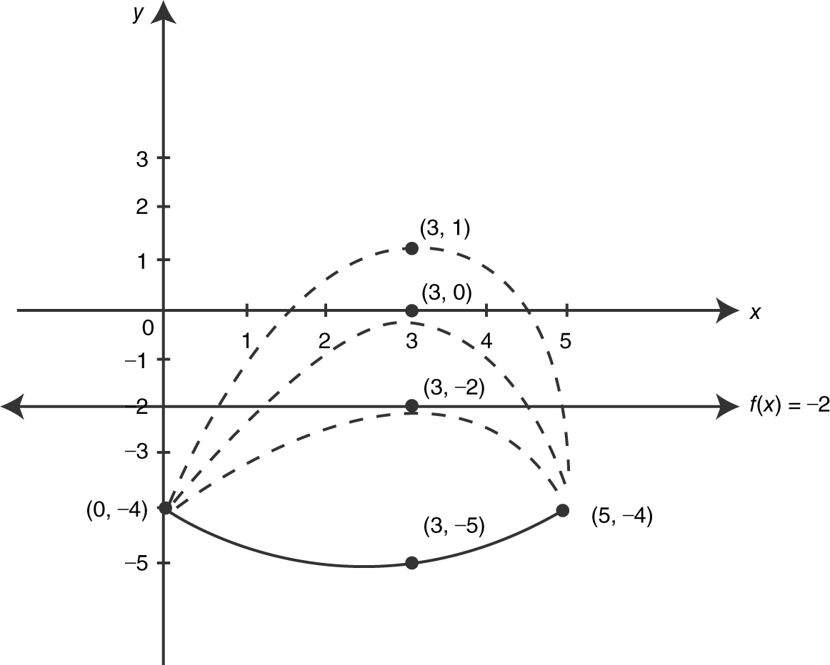
Figure 6.3-4

6.4 Rapid Review

1. Find f (2) and and determine if f is continuous at x = 2. (See Figure 6.4-1 .)

Answer: f (2) = 2, , and f is discontinuous at x = 2.

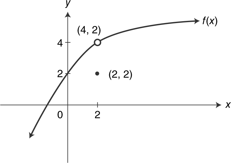
Figure 6.4-1

2. Evaluate

Answer: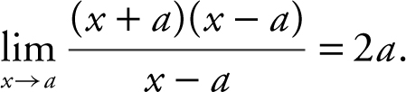

3. Evaluate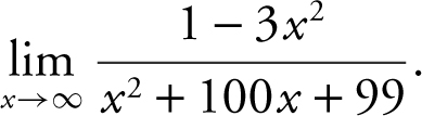

Answer: The limit is –3, since the polynomials in the numerator and denominator have the same degree.

4. Determine if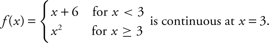

Answer: The function f is continuous, since f (3) = 9, f (x ) = 9, and .

5. If

Answer:

6. Evaluate

Answer: The limit is , since .

7. Evaluate .

Answer: The limit is –∞, since (x ² – 25) approaches 0 through negative values.

8. Find the vertical and horizontal asymptotes of .

Answer: The vertical asymptotes are x = ±5, and the horizontal asymptote is y = 0, since .

6.5 Practice Problems

Part A—The use of a calculator is not allowed.

Find the limits of the following:

1 .

2 . If b ≠ 0, evaluate .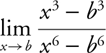

3 .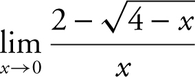

4 .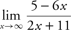

5 .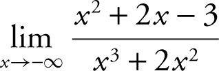

6 .

7 .

8 .

9 .

10 .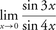

11 .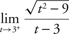

12 . The graph of a function f is shown in Figure 6.5-1 .
Which of the following statements is/are true?

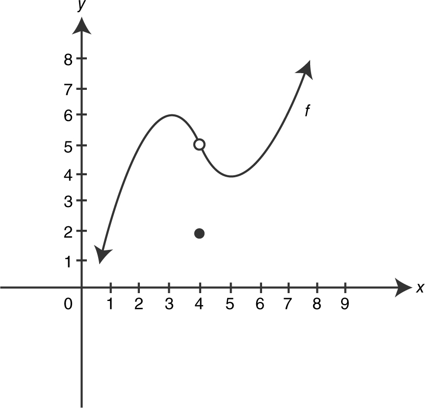
Figure 6.5-1

I.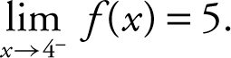

II.

III. x = 4 is not in the domain of f .

Part B—Calculators are allowed.

13 . Find the horizontal and vertical asymptotes of the graph of the function

.

14 . Find the limit: when [x ] is the greatest integer of x .

15 . Find all x -values where the function is discontinuous.

16 . For what value of k is the function 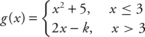continuous at x = 3?

17 . Determine if

is continuous at x = 2. Explain why or why not.

18 . Given f (x ) as shown in Figure 6.5-2 , find

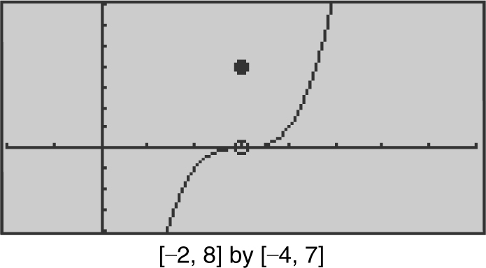
Figure 6.5-2

(a) f (3).

(b)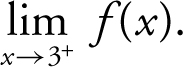

(c)

(d)

19 . A function f is continuous on [–2, 2] and some of the values of f are shown below:

If f has only one root, r , on the closed interval [–2, 2], and r ≠ 0, then a possible value of b is

(A) –2

(B) –1

(C) 0

(D) 1

20 . Evaluate .

6.6 Cumulative Review Problems

21 . Write an equation of the line passing through the point (2, –4) and perpendicular to the line 3x – 2y = 6.

22 . The graph of a function f is shown in Figure 6.6-1 . Which of the following statements is/are true?

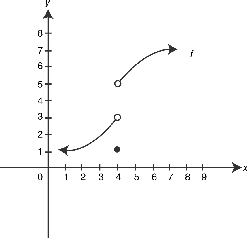
Figure 6.6-1

I.

II. x = 4 is not in the domain of f .

III. does not exist.

23 . Evaluate .

24 . Find .

25 . Find the horizontal and vertical asymptotes of .

6.7 Solutions to Practice Problems

Part A—The use of a calculator is not allowed.

1 . Using the product rule,

2 . Rewrite as 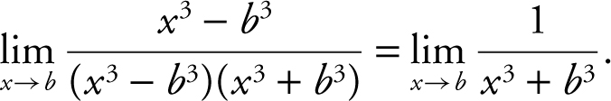Substitute x = b and obtain .

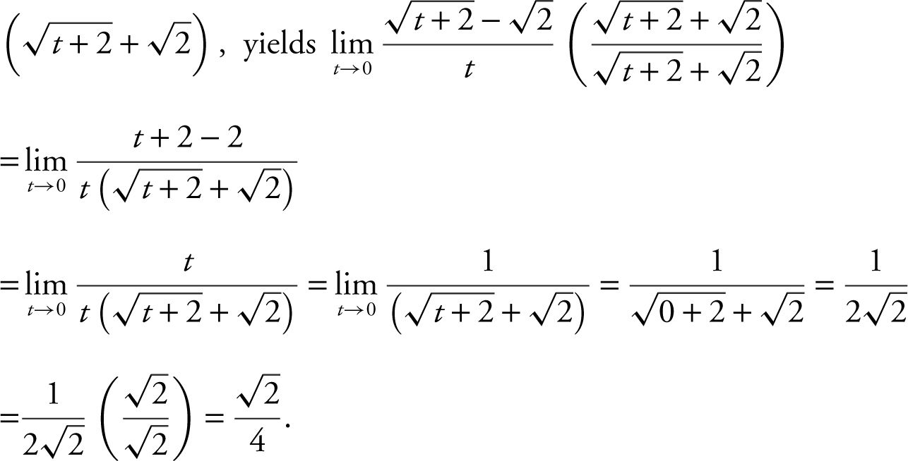
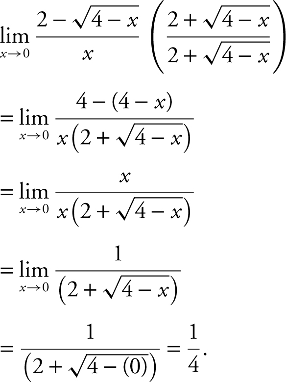
3 . Substituting x = 0 into the expression leads to 0/0 which is an indeterminate form. Thus, multiply both the numerator and denominator by the conjugate and obtain

4 . Since the degree of the polynomial in the numerator is the same as the degree of the polynomial in the denominator,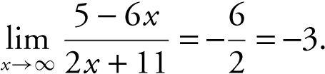

5 . Since the degree of the polynomial in the numerator is 2 and the degree of the polynomial in the denominator is 3,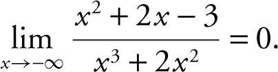

6 . The degree of the monomial in the numerator is 2 and the degree of the binomial in the denominator is 1. Thus,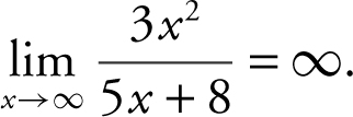

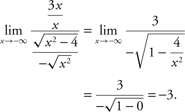
7 . Divide every term in both the numerator and denominator by the highest power of x . In this case, it is x . Thus, you have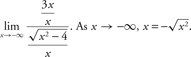

Since the denominator involves a radical, rewrite the expression as

8 .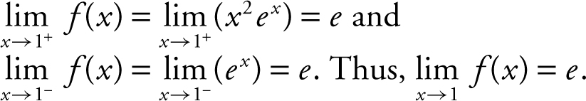

9 . 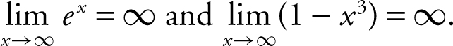. However, as x → ∞, the rate of increase of e ^x is much greater than the rate of decrease of (1 – x ³ ). Thus, .

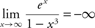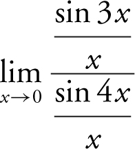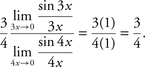
10 . Divide both numerator and denominator by x and obtain . Now rewrite the limit as 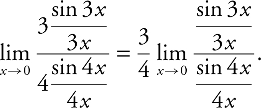. As x approaches 0, so do 3x and 4x .

Thus, you have

11 . As t → 3⁺ , (t – 3) > 0, and thus . Rewrite the limit as 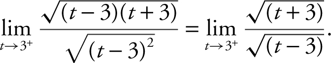The limit of the numerator is and the denominator is approaching 0 through positive values. Thus, positive values. Thus, .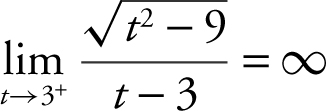

12 . The graph of f indicates that:

I. is true.

II. is false.
(The = 5.)

III. “x = 4 is not in the domain of f ” is false since f (4) = 2.

Part B—Calculators are allowed.

13 . Examining the graph in your calculator, you notice that the function approaches the x -axis as x → ∞ or as x → –∞. Thus, the line y = 0 (the x -axis) is a horizontal asymptote. As x approaches 1 from either side, the function increases or decreases without bound. Similarly, as x approaches –2 from either side, the function increases or decreases without bound. Therefore, x = 1 and x = –2 are vertical asymptotes. (See Figure 6.7-1 .)

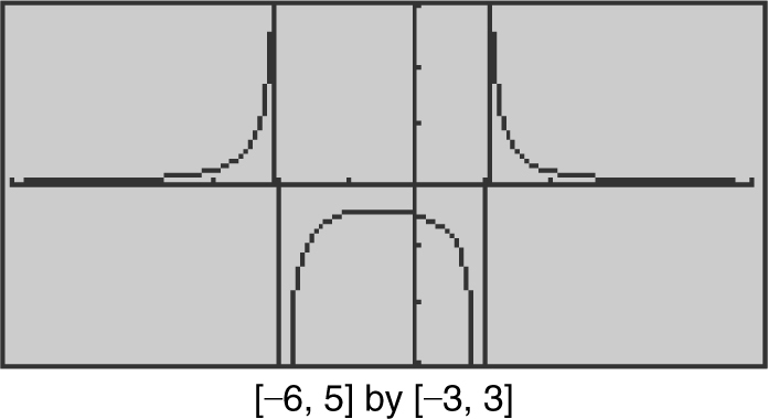
Figure 6.7-1

14 . As x → 5⁺ , the limit of the numerator (5 + [5]) is 10 and as x → 5⁺ , the denominator approaches 0 through negative values. Thus, the .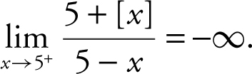

15 . Since f (x ) is a rational function, it is continuous everywhere except at values where the denominator is 0. Factoring and setting the denominator equal to 0, you have (x + 6) (x – 2) = 0. Thus, the function is discontinuous at x = –6 and x = 2. Verify your result with a calculator. (See Figure 6.7-2 .)

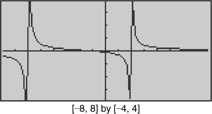
Figure 6.7-2

16 . In order for g (x ) to be continuous at x = 3, it must satisfy the three conditions of continuity:

(1) g (3) = 3² + 5 = 14,

(2) = 14, and

(3) – k , and the two one-sided limits must be equal in order for to exist. Therefore, 6 – k = 14 and k = –8.

Now, and condition 3 is satisfied.

17 . Checking with the three conditions of continuity:

(1) f (2) = 12,

(2)

, and
(3) . Therefore, f (x ) is discontinuos at x = 2.

18 . The graph indicates that (a) f (3) = 4, (b) , (c) , (d) , and (e) therefore, f (x ) is not continuous at x = 3 since .

19 . (See Figure 6.7-3 .) If b = 0, then r = 0, but r cannot be 0. If b = –3, –2, or –1, f would have more than one root. Thus b = 1. Choice (D).

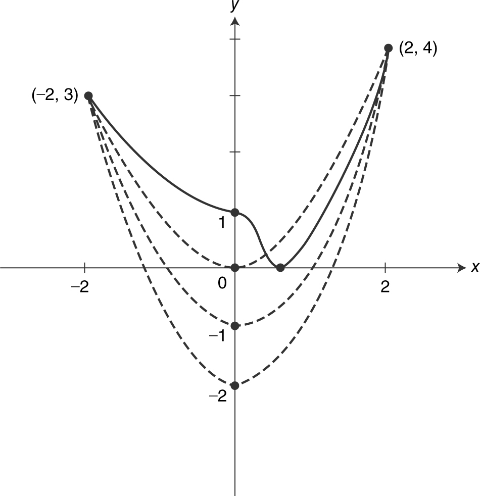
Figure 6.7-3

20 . Substituting x = 0 would lead to 0/0. Substitute (1 – cos² x ) in place of sin² x and obtain

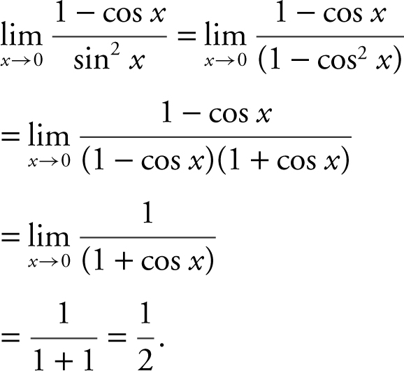
Verify your result with a calculator. (See Figure 6.7-4 )

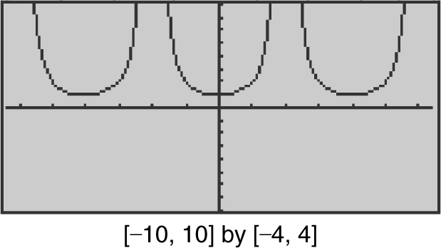
Figure 6.7-4

6.8 Solutions to Cumulative Review Problems

21 . Rewrite 3x – 2y = 6 in y = mx + b form which is . The slope of this line whose equation is is . Thus, the slope of a line perpendicular to this line is . Since the perpendicular line passes through the point (2, –4), therefore, an equation of the perpendicular line is which is equivalent to .

22 . The graph indicates that , f (4) = 1, and does not exist. Therefore, only statements I and III are true.

23 . Substituting x = 0 into , you obtain .

24 . Rewrite which is equivalent to which is equal to .

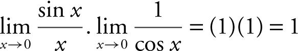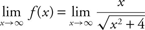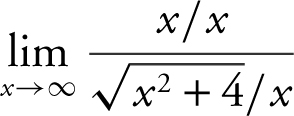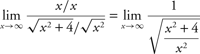
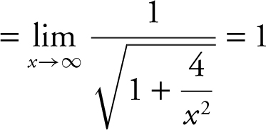25 . To find horizontal asymptotes, examine the and the . The . Dividing by the highest power of x (and in this case, it’s x ), you obtain . As x → ∞, . Thus, you have . Thus, the line y = 1 is a horizontal asymptote.

The 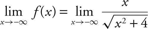. As . Thus, .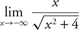

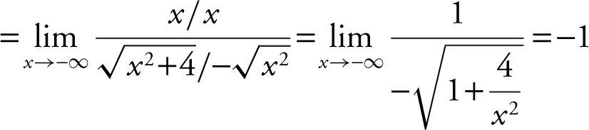Therefore, the line y = –1 is a horizontal asymptote. As for vertical asymptotes, f (x ) is continuous and defined for all real numbers. Thus, there is no vertical asymptote.