Calculus AB and Calculus BC
Introduction
This book is intended for students who are preparing to take either of the two Advanced Placement Examinations in Mathematics offered by the College Entrance Examination Board, and for their teachers. It is based on the May 2012 course description published by the College Board, and covers the topics listed there for both Calculus AB and Calculus BC.
Candidates who are planning to take the CLEP Examination on Calculus with Elementary Functions are referred to the section of this Introduction on that examination.
THE COURSES
Calculus AB and BC are both full-year courses in the calculus of functions of a single variable. Both courses emphasize:
(1) student understanding of concepts and applications of calculus over manipulation and memorization;
(2) developing the student’s ability to express functions, concepts, problems, and conclusions analytically, graphically, numerically, and verbally, and to understand how these are related; and
(3) using a graphing calculator as a tool for mathematical investigations and for problem-solving.
Both courses are intended for those students who have already studied college-preparatory mathematics: algebra, geometry, trigonometry, analytic geometry, and elementary functions (linear, polynomial, rational, exponential, logarithmic, trigonometric, inverse trigonometric, and piecewise). The AB topical course outline that follows can be covered in a full high-school academic year even if some time is allotted to studying elementary functions. The BC course assumes that students already have a thorough knowledge of all the topics noted above.
TOPICS THAT MAY BE TESTED ON THE CALCULUS AB EXAM
1. Functions and Graphs
Rational, trigonometric, inverse trigonometric, exponential, and logarithmic functions.
2. Limits and Continuity
Intuitive definitions; one-sided limits; functions becoming infinite; asymptotes and graphs; indeterminate limits of the form ![]() estimating limits using tables or graphs.
estimating limits using tables or graphs.
Definition of continuity; kinds of discontinuities; theorems about continuous functions; Extreme Value and Intermediate Value Theorems.
3. Differentiation
Definition of derivative as the limit of a difference quotient and as instantaneous rate of change; derivatives of power, exponential, logarithmic, trig and inverse trig functions; product, quotient, and chain rules; differentiability and continuity; estimating a derivative numerically and graphically; implicit differentiation; derivative of the inverse of a function; the Mean Value Theorem; recognizing a given limit as a derivative.
4. Applications of Derivatives
Rates of change; slope; critical points; average velocity; tangents and normals; increasing and decreasing functions; using the first and second derivatives for the following: local (relative) max or min, concavity, inflection points, curve sketching, global (absolute) max or min and optimization problems; relating a function and its derivatives graphically; motion along a line; local linearization and its use in approximating a function; related rates; differential equations and slope fields.
5. The Definite Integral
Definite integral as the limit of a Riemann sum; area; definition of definite integral; properties of the definite integral; Riemann sums using rectangles or sums using trapezoids; comparing approximating sums; average value of a function; Fundamental Theorem of Calculus; graphing a function from its derivative; estimating definite integrals from tables and graphs; accumulated change as integral of rate of change.
6. Integration
Antiderivatives and basic formulas; antiderivatives by substitution; applications of antiderivatives; separable differential equations; motion problems.
7. Applications of Integration to Geometry
Area of a region, including between two curves; volume of a solid of known cross section, including a solid of revolution.
8. Further Applications of Integration and Riemann Sums
Velocity and distance problems involving motion along a line; other applications involving the use of integrals of rates as net change or the use of integrals as accumulation functions; average value of a function over an interval.
9. Differential Equations
Basic definitions; geometric interpretations using slope fields; solving first-order separable differential equations analytically; exponential growth and decay.
TOPICS THAT MAY BE TESTED ON THE CALCULUS BC EXAM
BC ONLY
Any of the topics listed above for the Calculus AB exam may be tested on the BC exam. The following additional topics are restricted to the BC exam.
1. Functions and Graphs
Parametrically defined functions; polar functions; vector functions.
2. Limits and Continuity
No additional topics.
3. Differentiation
Derivatives of polar, vector, and parametrically defined functions; indeterminate forms; L’Hôpital’s rule.
4. Applications of Derivatives
Tangents to parametrically defined curves; slopes of polar curves; analysis of curves defined parametrically or in polar or vector form.
5. The Definite Integral
Integrals involving parametrically defined functions.
6. Integration
By parts; by partial fractions (involving nonrepeating linear factors only); improper integrals.
7. Applications of Integration to Geometry
Area of a region bounded by parametrically defined or polar curves; arc length.
8. Further Applications of Integration and Riemann Sums
Velocity and distance problems involving motion along a planar curve; velocity and acceleration vectors.
9. Differential Equations
Euler’s method; applications of differential equations, including logistic growth.
10. Sequences and Series
Definition of series as a sequence of partial sums and of its convergence as the limit of that sequence; harmonic, geometric, and p-series; integral, ratio, and comparison tests for convergence; alternating series and error bound; power series, including interval and radius of convergence; Taylor polynomials and graphs; finding a power series for a function; MacLaurin and Taylor series; Lagrange error bound for Taylor polynomials; computations using series.
THE EXAMINATIONS
The Calculus AB and BC Examinations and the course descriptions are prepared by committees of teachers from colleges or universities and from secondary schools. The examinations are intended to determine the extent to which a student has mastered the subject matter of the course.
Each examination is 3 hours and 15 minutes long, as follows:
Section I has two parts. Part A has 28 multiple-choice questions for which 55 minutes are allowed. The use of calculators is not permitted in Part A.
Part B has 17 multiple-choice questions for which 50 minutes are allowed. Some of the questions in Part B require the use of a graphing calculator.
Section II, the free-response section, has a total of six questions in two parts:
Part A has two questions, of which some parts require the use of a graphing calculator. After 30 minutes, however, you will no longer be permitted to use a calculator. If you finish Part A early, you will not be permitted to start work on Part B.
Part B has four questions and you are allotted an additional 60 minutes, but you are not allowed to use a calculator. You may work further on the Part A questions (without your calculator).
The section that follows gives important information on its use (and misuse!) of the graphing calculator.
THE GRAPHING CALCULATOR: USING YOUR GRAPHING CALCULATOR ON THE AP EXAM
The Four Calculator Procedures
Each student is expected to bring a graphing calculator to the AP Exam. Different models of calculators vary in their features and capabilities; however, there are four procedures you must be able to perform on your calculator:
C1. Produce the graph of a function within an arbitrary viewing window.
C2. Solve an equation numerically.
C3. Compute the derivative of a function numerically.
C4. Compute definite integrals numerically.
Guidelines for Calculator Use
1. On multiple-choice questions in Section I, Part B, you may use any feature or program on your calculator. Warning: Don’t rely on it too much! Only a few of these questions require the calculator, and in some cases using it may be too time-consuming or otherwise disadvantageous.
2. On the free-response questions of Section II Part A:
(a) You may use the calculator to perform any of the four listed procedures. When you do, you need only write the equation, derivative, or definite integral (called the “setup”) that will produce the solution, then write the calculator result to the required degree of accuracy (three places after the decimal point unless otherwise specified). Note especially that a setup must be presented in standard algebraic or calculus notation, not just in calculator syntax. For example, you must include in your work the setup ![]() even if you use your calculator to evaluate the integral.
even if you use your calculator to evaluate the integral.
(b) For a solution for which you use a calculator capability other than the four listed above, you must write down the mathematical steps that yield the answer. A correct answer alone will not earn full credit.
(c) You must provide mathematical reasoning to support your answer. Calculator results alone will not be sufficient.
The Procedures Explained
Here is more detailed guidance for the four allowed procedures.
C1. “Produce the graph of a function within an arbitrary viewing window.” Be sure that you create the graph in the window specified, then copy it carefully onto your exam paper. If no window is prescribed in the question, clearly indicate the window dimensions you have used.
C2. “Solve an equation numerically” is equivalent to “Find the zeros of a function” or “Find the point of intersection of two curves.” Remember: you must first show your setup—write the equation out algebraically; then it is sufficient just to write down the calculator solution.
C3. “Compute the derivative of a function numerically.” When you seek the value of the derivative of a function at a specific point, you may use your calculator. First, indicate what you are finding—for example, f ′(6)—then write the numerical answer obtained from your calculator. Note that if you need to find the derivative itself, rather than its value at a particular point, you must show how you obtained it and what it is, even though some calculators are able to perform symbolic operations.
C4. “Compute definite integrals numerically.” If, for example, you need to find the area under a curve, you must first show your setup. Write the complete integral, including the integrand in terms of a single variable and with the limits of integration. You may then simply write the calculator answer; you need not compute an antiderivative.
Sample Solutions of Free-Response Questions
The following set of examples illustrates proper use of your calculator on the examination. In all of these examples, the function is
![]()
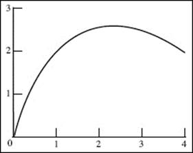
Viewing window [0,4] × [0,3].
1. Graph f in [0,4] × [0,3].
Set the calculator window to the dimensions printed in your exam paper.
Graph ![]()
Copy your graph carefully into the window on the exam paper.
2. Write the local linearization for f(x) near x = 1.
Note that f (1) = 2. Then, using your calculator, evaluate the derivative:
f ′(1) = 1.2
Then write the tangent-line (or local linear) approximation
![]()
You need not simplify, as we have, after the last equals sign just above.
3. Find the coordinates of any maxima of f. Justify your answer.
Since finding a maximum is not one of the four allowed procedures, you must use calculus and show your work, writing the derivative algebraically and setting it equal to zero to find any critical numbers:
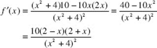
Then f ′(x) = 0 at x = 2 and at x = −2; but −2 is not in the specified domain.
We analyze the signs of f ′(which is easier here than it would be to use the second-derivative test) to assure that x = 2 does yield a maximum for f. (Note that the signs analysis alone is not sufficient justification.)
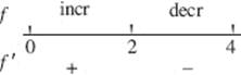
Since f ′ is positive to the left of x = 2 and negative to the right of x = 2, f does have a maximum at
![]()
—but you may leave f (2) in its unsimplified form, without evaluating to ![]()
You may use your calculator’s maximum-finder to verify the result you obtain analytically, but that would not suffice as a solution or justification.
4. Find the x-coordinate of the point where the line tangent to the curve y = f (x) is parallel to the secant on the interval [0,4].
Since f (0) = 0 and f (4) = 2, the secant passes through (0,0) and (4,2) and has slope ![]()
To find where the tangent is parallel to the secant, we find f ′(x) as in Example 3. We then want to solve the equation
![]()
The last equality above is the setup; we use the calculator to solve the equation: x = 1.458 is the desired answer.
5. Estimate the area under the curve y = f (x) using the Trapezoid Rule with four equal subintervals.
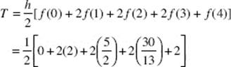
You may leave the answer in this form or simplify it to 7.808. If your calculator has a program for the Trapezoid Rule, you may use it to complete the computation after you have shown the setup as in the two equations above. If you omit them you will lose credit.
6. Find the volume of the solid generated when the curve y = f (x) on [0,4] is rotated about the x-axis.
Using disks, we have
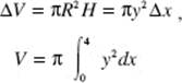
Note that the equation above is not yet the setup: the definite integral must be in terms of x alone:
![]()
Now we have shown the setup. Using the calculator we can evaluate V:
V = 55.539
A Note About Solutions in This Book
Students should be aware that in this book we sometimes do not observe the restrictions cited above on the use of the calculator. In providing explanations for solutions to illustrative examples or to exercises we often exploit the capabilities of the calculator to the fullest. Indeed, students are encouraged to do just that on any question of Section I, Part B, of the AP examination for which they use a calculator. However, to avoid losing credit, you must carefully observe the restrictions imposed on when and how the calculator may be used in answering questions in Section II of the examination.
Additional Notes and Reminders
• SYNTAX. Learn the proper syntax for your calculator: the correct way to enter operations, functions, and other commands. Parentheses, commas, variables, or parameters that are missing or entered in the wrong order can produce error messages, waste time, or (worst of all) yield wrong answers.
• RADIANS. Keep your calculator set in radian mode. Almost all questions about angles and trigonometric functions use radians. If you ever need to change to degrees for a specific calculation, return the calculator to radian mode as soon as that calculation is complete.
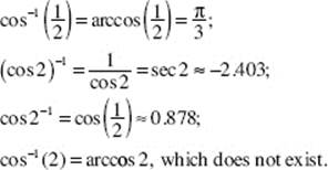
• TRIGONOMETRIC FUNCTIONS. Many calculators do not have keys for the secant, cosecant, or cotangent function. To obtain these functions, use their reciprocals.
For example, ![]()
Evaluate inverse functions such as arcsin, arccos, and arctan on your calculator. Those function keys are usually denoted as sin−1, cos−1, and tan−1.
Don’t confuse reciprocal functions with inverse functions. For example:
• NUMERICAL DERIVATIVES. You may be misled by your calculator if you ask for the derivative of a function at a point where the function is not differentiable, because the calculator evaluates numerical derivatives using the difference quotient (or the symmetric difference quotient). For example, if f (x) = |x|, then f ′(0) does not exist. Yet the calculator may find the value of the derivative as
![]()
Remember: always be sure f is differentiable at a before asking for f ′(a).
• IMPROPER INTEGRALS. Most calculators can compute only definite integrals. Avoid using yours to obtain an improper integral, such as
![]()
• ROUNDING-OFF ERRORS. To achieve three-place accuracy in a final answer, do not round off numbers at intermediate steps, since this is likely to produce error-accumulations. If necessary, store longer intermediate answers internally in the calculator; do not copy them down on paper (storing is faster and avoids transcription errors). Round off only after your calculator produces the final answer.
• ROUNDING THE FINAL ANSWER: UP OR DOWN? In rounding to three decimal places, remember that whether one rounds down or up depends on the nature of the problem. The mechanical rule followed in accounting (anything less than 0.0005 is rounded down, anything equal to or greater than 0.0005 is rounded up) does not apply.
Suppose, for example, that a problem seeks the largest k, to three decimal places, for which a condition is met, and the unrounded answer is 0.1239 …. Then 0.124 is too large: it does not meet the condition. The rounded answer must be 0.123. However, suppose that an otherwise identical problem seeks the smallest k for which a condition is met. In this case 0.1239 meets the condition but 0.1238 does not, so the rounding must be up, to 0.124.
• FINAL ANSWERS TO SECTION II QUESTIONS. Although we usually express a final answer in this book in simplest form (often evaluating it on the calculator), this is hardly ever necessary on Section II questions of the AP Examination. According to the directions printed on the exam, “unless otherwise specified” (1) you need not simplify algebraic or numerical answers; (2) answers involving decimals should be correct to three places after the decimal point. However, be aware that if you try to simplify, you must do so correctly or you will lose credit.
• USE YOUR CALCULATOR WISELY. Bear in mind that you will not be allowed to use your calculator at all on Part A of Section I. In Part B of Section I and part of Section II only a few questions will require one. As repeated often in this section, the questions that require a calculator will not be identified. You will have to be sensitive not only to when it is necessary to use the calculator but also to when it is efficient to do so.
The calculator is a marvelous tool, capable of illustrating complicated concepts with detailed pictures and of performing tasks that would otherwise be excessively time-consuming—or even impossible. But the completion of calculations and the displaying of graphs on the calculator can be slow. Sometimes it is faster to find an answer using arithmetic, algebra, and analysis without recourse to the calculator. Before you start pushing buttons, take a few seconds to decide on the best way to attack a problem.
GRADING THE EXAMINATIONS
Each completed AP examination paper receives a grade according to the following five-point scale:
5. Extremely well qualified
4. Well qualified
3. Qualified
2. Possibly qualified
1. No recommendation
SCORING CHANGE
In 2011 The College Board changed how the AP Calculus exams are scored. There is no penalty for wrong answers in the multiple-choice section.
Many colleges and universities accept a grade of 3 or better for credit or advanced placement or both; some also consider a grade of 2, while others require a grade of 4. (Students may check AP credit policies at individual colleges’ websites.) More than 59 percent of the candidates who took the 2012 Calculus AB Examination earned grades of 3, 4, or 5. More than 82 percent of the 2012 BC candidates earned 3 or better. More than 356,000 students altogether took the 2012 mathematics examination.
The multiple-choice questions in Section I are scored by machine. Students should note that the score will be the number of questions answered correctly. Since no points can be earned if answers are left blank and there is no deduction for wrong answers, students should answer every question. For questions they cannot do, students should try to eliminate as many of the choices as possible and then pick the best remaining answer.
The problems in Section II are graded by college and high-school teachers called “readers.” The answers in any one examination booklet are evaluated by different readers, and for each reader all scores given by preceding readers are concealed, as are the student’s name and school. Readers are provided sample solutions for each problem, with detailed scoring scales and point distributions that allow partial credit for correct portions of a student’s answer. Problems in Section II are all counted equally.
In the determination of the overall grade for each examination, the two sections are given equal weight. The total raw score is then converted into one of the five grades listed above. Students should not think of these raw scores as percents in the usual sense of testing and grading. A student who averages 6 out of 9 points on the Section II questions and performs similarly well on Section I’s multiple-choice questions will typically earn a 5. Many colleges offer credit for a score of 3, historically awarded for earning over 40 of 108 possible points.
Students who take the BC examination are given not only a Calculus-BC grade but also a Calculus-AB subscore grade. The latter is based on the part of the BC examination dealing with topics in the AB syllabus.
In general, students will not be expected to answer all the questions correctly in either Section I or II.
Great care is taken by all involved in the scoring and reading of papers to make certain that they are graded consistently and fairly so that a student’s overall AP grade reflects as accurately as possible his or her achievement in calculus.
THE CLEP CALCULUS EXAMINATION
Many colleges grant credit to students who perform acceptably on tests offered by the College Level Examination Program (CLEP). The CLEP calculus examination is one such test.
The College Board’s CLEP Official Study Guide: 16th Edition provides descriptions of all CLEP examinations, test-taking tips, and suggestions on reference and supplementary materials. According to the Guide, the calculus examination covers topics usually taught in a one-semester college calculus course. It is assumed that students taking the exam will have studied college-preparatory mathematics (algebra, plane and solid geometry, analytic geometry, and trigonometry).
There are 45 multiple-choice questions on the CLEP calculus exam, for which 90 minutes are allowed. A calculator may not be used during the examination.
Approximately 60 percent of the questions are on limits and differential calculus and about 40 percent on integral calculus. The specific topics that may be tested on the CLEP calculus exam are essentially those under the heading “Topics That May Be Tested on the Calculus AB Exam.” (L’Hôpital’s Rule is listed as a CLEP calculus topic but only as a BC topic for the AP exam. Also, the only topics listed as applications of the definite integral for the CLEP calculus test are “average value of a function on an interval” and “area.”)
Since any topic that may be tested on the CLEP calculus exam is included in this book on the AP Exam, a candidate who plans to take the CLEP exam will benefit from a review of the AB topics covered here. The multiple-choice questions in Part A of Chapter 11 and in Part A of Section I of each of the four AB Practice Examinations will provide good models for questions on the CLEP calculus test.
A complete description of the knowledge and skills required and of the specific topics that may be tested on the CLEP exam can be downloaded from the College Board’s web site at www.collegeboard.com/clep.
THIS REVIEW BOOK
This book consists of the following parts:
Diagnostic tests for both AB and BC Calculus are practice AP exams. They are followed by solutions keyed to the corresponding topical review chapter.
Topical Review and Practice includes 10 chapters with notes on the main topics of the Calculus AB and BC syllabi and with numerous carefully worked-out examples. Each chapter concludes with a set of multiple-choice questions, usually divided into calculator and no-calculator sections, followed immediately by answers and solutions.
This review is followed by further practice: (1) Chapter 11, which includes a set of multiple-choice questions on miscellaneous topics and an answer key; (2) Chapter 12, a set of miscellaneous free-response problems that are intended to be similar to those in Section II of the AP examinations. They are followed by solutions.
The next part of the book, titled Practice Examinations: Sections I and II, has three AB and three BC practice exams that simulate the actual AP examinations. Each is followed by answers and explanations.
In this book, review material on topics covered only in Calculus BC is preceded by an asterisk (*), as are both multiple-choice questions and free-response-type problems that are likely to occur only on a BC Examination.
THE TEACHER WHO USES THIS BOOK WITH A CLASS may profitably do so in any of several ways. If the book is used throughout a year’s course, the teacher can assign all or part of each set of multiple-choice questions and some miscellaneous exercises after the topic has been covered. These sets can also be used for review purposes shortly before examination time. The Practice Examinations will also be very helpful in reviewing toward the end of the year. Teachers may also assemble examinations by choosing appropriate problems from the sample Miscellaneous Practice Questions in Chapters 11 and 12.
STUDENTS WHO USE THIS BOOK INDEPENDENTLY will improve their performance by studying the illustrative examples carefully and trying to complete practice problems before referring to the solution keys.
Since many FIRST-YEAR MATHEMATICS COURSES IN COLLEGES follow syllabi much like that proposed by the College Board for high-school Advanced Placement courses, college students and teachers may also find the book useful.
FLASH CARDS
Being able to answer AP exam questions quickly and correctly depends in part on knowing many fundamental facts, such as
• common math formulas (e.g., area, volume, trig identities);
• definitions of key terms (e.g., continuous, differentiable, integrable);
• important theorems (e.g., Mean Value Theorem, Fundamental Theorem of Calculus); and
• derivatives and antiderivatives of common functions.
Barron’s AP Calculus Flash Cards (ISBN 9780764194214) provide a great way to study these facts and more. Over 300 cards will help you learn the most important information you’ll need to know for the AP Calculus examination.