Calculus AB and Calculus BC

CHAPTER 2 Limits and Continuity

F. CONTINUITY

If a function is continuous over an interval, we can draw its graph without lifting pencil from paper. The graph has no holes, breaks, or jumps on the interval.

Conceptually, if f (x) is continuous at a point x = c, then the closer x is to c, the closer f (x) gets to f (c). This is made precise by the following definition:

DEFINITION

The function y = f (x) is continuous at x = c if

(1) f (c) exists; (that is, c is in the domain of f );

(2) exists;

(3)

A function is continuous over the closed interval [a, b] if it is continuous at each x such that a ≤ x ≤ b.

A function that is not continuous at x = c is said to be discontinuous at that point. We then call x = c a point of discontinuity.

CONTINUOUS FUNCTIONS

Polynomials are continuous everywhere; namely, at every real number.

Rational functions, are continuous at each point in their domain; that is, except where Q(x) = 0. The function for example, is continuous except at x = 0, where f is not defined.

The absolute value function f (x) = |x| (sketched in Figure N2–3) is continuous everywhere.

The trigonometric, inverse trigonometric, exponential, and logarithmic functions are continuous at each point in their domains.

Functions of the type (where n is a positive integer ≥ 2) are continuous at each x for which is defined.

The greatest-integer function f (x) = [x] (Figure N2–1) is discontinuous at each integer, since it does not have a limit at any integer.

KINDS OF DISCONTINUITIES

In Example 2, y = f (x) is defined as follows:

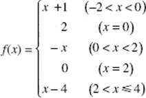
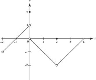
The graph of f is shown above.

We observe that f is not continuous at x = −2, x = 0, or x = 2.

At x = −2, f is not defined.

At x = 0, f is defined; in fact, f (0) = 2. However, since and does not exist. Where the left- and right-hand limits exist, but are different, the function has a jump discontinuity. The greatest-integer (or step) function, y = [x], has a jump discontinuity at every integer.

At x = 2, f is defined; in fact, f (2) = 0. Also, the limit exists. However, This discontinuity is called removable. If we were to redefine the function at x = 2 to be f (2) = −2, the new function would no longer have a discontinuity there. We cannot, however, “remove” a jump discontinuity by any redefinition whatsoever.

Whenever the graph of a function f (x) has the line x = a as a vertical asymptote, then f (x) becomes positively or negatively infinite as x → a⁺ or as x → a⁻. The function is then said to have an infinite discontinuity. See, for example, Figure N2–4 for Figure N2–5 for or Figure N2–7 for Each of these functions exhibits an infinite discontinuity.

EXAMPLE 24

is not continuous at x = 0 or = −1, since the function is not defined for either of these numbers. Note also that neither nor exists.

EXAMPLE 25

Discuss the continuity of f, as graphed in Figure N2–9.

SOLUTION: f (x) is continuous on [(0,1), (1,3), and (3,5)]. The discontinuity at x = 1 is removable; the one at x = 3 is not. (Note that f is continuous from the right at x = 0 and from the left at x = 5.)

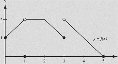
FIGURE N2–9

In Examples 26 through 31, we determine whether the functions are continuous at the points specified:

EXAMPLE 26

Is continuous at x = −1?

SOLUTION: Since f is a polynomial, it is continuous everywhere, including, of course, at x = −1.

EXAMPLE 27

Is continuous (a) at x = 3; (b) at x = 0?

SOLUTION: This function is continuous except where the denominator equals 0 (where g has an infinite discontinuity). It is not continuous at x = 3, but is continuous at x = 0.

EXAMPLE 28

Is 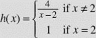continuous

(a) at x = 2; (b) at x = 3?

SOLUTIONS:

(a) h(x) has an infinite discontinuity at x = 2; this discontinuity is not removable.

(b) h(x) is continuous at x = 3 and at every other point different from 2. See Figure N2–10.

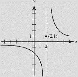
FIGURE N2–10

EXAMPLE 29

Is (x ≠ 2) continuous at x = 2?

SOLUTION: Note that k(x) = x + 2 for all x ≠ 2. The function is continuous everywhere except at x = 2, where k is not defined. The discontinuity at 2 is removable. If we redefine f (2) to equal 4, the new function will be continuous everywhere. See Figure N2–11.

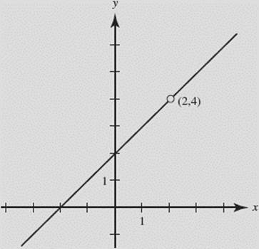
FIGURE N2–11

EXAMPLE 30

Is 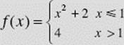continuous at x = 1?

SOLUTION: f (x) is not continuous at x = 1 since This function has a jump discontinuity at x = 1 (which cannot be removed). See Figure N2–12.

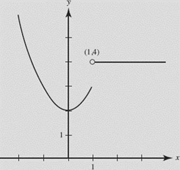
FIGURE N2–12

EXAMPLE 31

Is 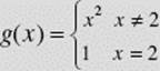continuous at x = 2?

SOLUTION: g(x) is not continuous at x = 2 since This discontinuity can be removed by redefining g(2) to equal 4. See Figure N2–13.

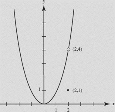
FIGURE N2–13

THEOREMS ON CONTINUOUS FUNCTIONS

(1) The Extreme Value Theorem. If f is continuous on the closed interval [a,b], then f attains a minimum value and a maximum value somewhere in that interval.

(2) The Intermediate Value Theorem. If f is continuous on the closed interval [a,b], and M is a number such that f (a) ≤ M ≤ f (b), then there is at least one number, c, between a and b such that f (c) = M.

Note an important special case of the Intermediate Value Theorem:

If f is continuous on the closed interval [a,b], and f (a) and f (b) have opposite signs, then f has a zero in that interval (there is a value, c, in [a,b] where f (c) = 0).

(3) The Continuous Functions Theorem. If functions f and g are both continuous at x = c, then so are the following functions:

(a) kf, where k is a constant;

(b) f ± g;

(c) f · g;

(d) provided that g(c) ≠ 0.

EXAMPLE 32

Show that 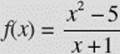has a root between x = 2 and x = 3.

SOLUTION: The rational function f is discontinuous only at and f (3) = 1. Since f is continuous on the interval [2,3] and f (2) and f (3) have opposite signs, there is a value, c, in the interval where f (c) = 0, by the Intermediate Value Theorem.

Chapter Summary

In this chapter, we have reviewed the concept of a limit. We’ve practiced finding limits using algebraic expressions, graphs, and the Squeeze (Sandwich) Theorem. We have used limits to find horizontal and vertical asymptotes and to assess the continuity of a function. We have reviewed removable, jump, and infinite discontinuities. We have also looked at the very important Extreme Value Theorem and Intermediate Value Theorem.