Calculus AB and Calculus BC

CHAPTER 3 Differentiation

E. ESTIMATING A DERIVATIVE

E1. Numerically.

EXAMPLE 22

The table shown gives the temperatures of a polar bear on a very cold arctic day (t = minutes; T = degrees Fahrenheit):

Our task is to estimate the derivative of T numerically at various times. A possible graph of T(t) is sketched in Figure N3–3, but we shall use only the data from the table.

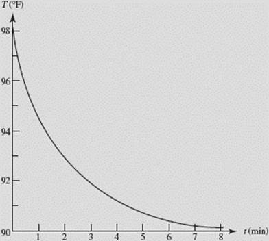
FIGURE N3–3

Using the difference quotient with h equal to 1, we see that

Also,

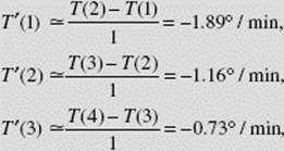
and so on.

The following table shows the approximate values of T ′(t) obtained from the difference quotients above:

Note that the entries for T ′(t) also represent the approximate slopes of the T curve at times 0.5, 1.5, 2.5, and so on.

From a Symmetric Difference Quotient

In Example 22 we approximated a derivative numerically from a table of values. We can also estimate f ′(a) numerically using the symmetric difference quotient, which is defined as follows:

Note that the symmetric difference quotient is equal to

We see that it is just the average of two difference quotients. Many calculators use the symmetric difference quotient in finding derivatives.

EXAMPLE 23

For the function f (x) = x⁴, approximate f ′(1) using the symmetric difference quotient with h = 0.01.

SOLUTION:

The exact value of f ′(1), of course, is 4.

The use of the symmetric difference quotient is particularly convenient when, as is often the case, obtaining a derivative precisely (with formulas) is cumbersome and an approximation is all that is needed for practical purposes.

A word of caution is in order. Sometimes a wrong result is obtained using the symmetric difference quotient. We noted that f (x) = |x| does not have a derivative at x = 0, since f ′(x) = −1 for all x < 0 but f ′(x) = 1 for all x > 0. Our calculator (which uses the symmetric difference quotient) tells us (incorrectly!) that f ′(0) = 0. Note that, if f (x) = |x|, the symmetric difference quotient gives 0 for f ′(0) for every h ≠ 0. If, for example, h = 0.01, then we get

which, as previously noted, is incorrect. The graph of the derivative of f (x) = |x|, which we see in Figure N3–4, shows that f ′(0) does not exist.

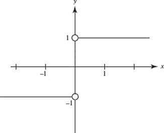
FIGURE N3–4

E2. Graphically.

If we have the graph of a function f (x), we can use it to graph f ′(x). We accomplish this by estimating the slope of the graph of f (x) at enough points to assure a smooth curve for f ′(x). In Figure N3–5 we see the graph of y = f (x). Below it is a table of the approximate slopes estimated from the graph.

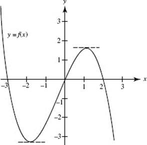
FIGURE N3–5

Figure N3–6 was obtained by plotting the points from the table of slopes above and drawing a smooth curve through these points. The result is the graph of y = f ′(x).

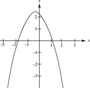
FIGURE N3–6

From the graphs above we can make the following observations:

(1) At the points where the slope of f (in Figure N3–5) equals 0, the graph of f ′(Figure N3–6) has x-intercepts: approximately x = −1.8 and x = 1.1. We’ve drawn horizontal broken lines at these points on the curve in Figure N3–5.

(2) On intervals where f the derivative is We see here that f decreases for x < −1.8 (approximately) and for x > 1.1 (approximately), and that f increases for −1.8 < x < 1.1 (approximately). In Chapter 4 we discuss other behaviors of f that are reflected in the graph of f ′.

BC ONLY