Calculus AB and Calculus BC
CHAPTER 6 Definite Integrals
G. AVERAGE VALUE
Average value of a function
If the function y = f (x) is integrable on the interval a ≤ x ≤ b, then we define the average value of f from a to b to be
![]()
Note that (1) is equivalent to
![]()
If f (x) ≥ 0 for all x on [a,b], we can interpret (2) in terms of areas as follows: The right-hand expression represents the area under the curve of y = f (x), above the x-axis, and bounded by the vertical lines x = a and x = b. The left-hand expression of (2) represents the area of a rectangle with the same base (b − a) and with the average value of f as its height. See Figure N6–17.
CAUTION: The average value of a function is not the same as the average rate of change. Before answering any question about either of these, be sure to reread the question carefully to be absolutely certain which is called for.
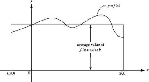
FIGURE N6–17
EXAMPLE 37
Find the average value of f (x) = ln x on the interval [1,4].
SOLUTION: ![]()
EXAMPLE 38
Find the average value of y for the semicircle ![]() on [−2,2].
on [−2,2].
SOLUTION: ![]()
NOTE: We have used the fact that the definite integral equals exactly the area of a semicircle of radius 2.
EXAMPLE 39
The graphs (a) through (e) in Figure N6–18 show the velocities of five cars moving along an east-west road (the x-axis) at time t, where 0 ≤ t ≤ 6. In each graph the scales on the two axes are the same.
Which graph shows the car
(1) with constant acceleration?
(2) with the greatest initial acceleration?
(3) back at its starting point when t = 6?
(4) that is furthest from its starting point at t = 6?
(5) with the greatest average velocity?
(6) with the least average velocity?
(7) farthest to the left of its starting point when t = 6?
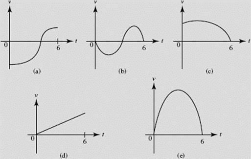
FIGURE N6–18
SOLUTIONS:
(1) (d), since acceleration is the derivative of velocity and in (d) v ′, the slope, is constant.
(2) (e), when t = 0 the slope of this v-curve (which equals acceleration) is greatest.
(3) (b), since for this car the net distance traveled (given by the net area) equals zero.
(4) (e), since the area under the v-curve is greatest, this car is farthest east.
(5) (e), the average velocity equals the total distance divided by 6, which is the net area divided by 6 (see (4)).
(6) (a), since only for this car is the net area negative.
(7) (a) again, since net area is negative only for this car.
EXAMPLE 40
Identify each of the following quantities for the function f (x), whose graph is shown in Figure N6–19a (note: F ′(x) = f (x)):
(a) f (b) − f (a)
(b) ![]()
(c) F(b) − F(a)
(d) ![]()
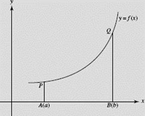
FIGURE N6–19a
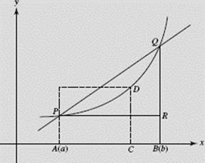
FIGURE N6–19b
SOLUTIONS: See Figure N6–19b.
(a) f (b) − f (a) = length RQ.
(b) ![]() = slope of secant PQ.
= slope of secant PQ.
(c) F(b) − F(a) = ![]() = area of APDQB.
= area of APDQB.
(d) ![]() = average value of f over [a,b] = length of CD, where CD · AB or CD · (b − a) is equal to the area F(b) − F(a).
= average value of f over [a,b] = length of CD, where CD · AB or CD · (b − a) is equal to the area F(b) − F(a).
EXAMPLE 41
The graph in Figure N6–20 shows the speed v(t) of a car, in miles per hour, at 10-minute intervals during a 1-hour period.
(a) Give an upper and a lower estimate of the total distance traveled.
(b) When does the acceleration appear greatest?
(c) Estimate the acceleration when t = 20.
(d) Estimate the average speed of the car during the interval 30 ≤ t ≤ 50.
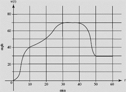
FIGURE N6–20
SOLUTIONS:
(a) A lower estimate, using minimum speeds and ![]() hr for 10 min, is
hr for 10 min, is
![]()
This yields ![]() mi for the total distance traveled during the hour. An upper estimate uses maximum speeds; it equals
mi for the total distance traveled during the hour. An upper estimate uses maximum speeds; it equals
![]()
or 55 mi for the total distance.
(b) The acceleration, which is the slope of v(t), appears greatest at t = 5 min, when the curve is steepest.
(c) To estimate the acceleration v ′(t) at t = 20, we approximate the slope of the curve at t = 20. The slope of the tangent at t = 20 appears to be equal to (10 mph)/(10 min) = (10 mph)/![]() = 60 mi/hr2.
= 60 mi/hr2.
(d) The average speed equals the distance traveled divided by the time. We can approximate the distance from t = 30 to t = 50 by the area under the curve, or, roughly, by the sum of the areas of a rectangle and a trapezoid:
![]()
Thus the average speed from t = 30 to t = 50 is
![]()
EXAMPLE 42
Given the graph of G(x) in Figure N6–21a, identify the following if G ′(x) = g(x):
(a) g(b)
(b) ![]()
(c) ![]()
(d) 
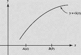
FIGURE N6–21a
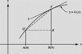
FIGURE N6–21b
SOLUTIONS: See Figure N6–21b.
(a) g(b) is the slope of G(x) at b, the slope of line ST.
(b) ![]() is equal to the area under G(x) from a to b.
is equal to the area under G(x) from a to b.
(c) ![]() = G(b) − G(a) = length of BT − length of BR = length of RT.
= G(b) − G(a) = length of BT − length of BR = length of RT.
(d) 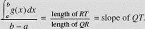
EXAMPLE 43
The function f (t) is graphed in Figure N6–22a. Let
![]()
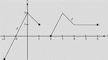
FIGURE N6–22a
(a) What is the domain of F ?
(b) Find x, if F ′(x) = 0.
(c) Find x, if F(x) = 0.
(d) Find x, if F(x) = 1.
(e) Find F ′(6).
(f) Find F(6).
(g) Sketch the complete graph of F.
SOLUTIONS:
(a) The domain of f is [−2,1] and [2,6], We choose the portion of this domain that contains the lower limit of integration, 4. Thus the domain of
F is 2 ≤ ![]() ≤ 6, or 4 ≤ x ≤ 12.
≤ 6, or 4 ≤ x ≤ 12.
(b) Since ![]()
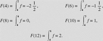
(c) F(x) = 0 when ![]() or x = 8. F(8) =
or x = 8. F(8) = ![]()
(d) For F(x) to equal 1, we need a region under f whose left endpoint is 4 with area equal to 1. The region from 4 to 5 works nicely; so ![]() and x = 10.
and x = 10.
(e) ![]()
(f) F(6) = ![]()
(g) In Figure N6–22b we evaluate the areas in the original graph.
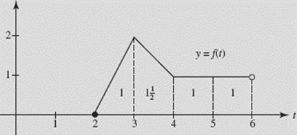
FIGURE N6–22b
Measured from the lower limit of integration, 4, we have (with “f” as an abbreviation for “f (t) dt”):
We note that, since F ′(= f ) is linear on (2,4), F is quadratic on (4,8); also, since F ′ is positive and increasing on (2,3), the graph of F is increasing and concave up on (4,6), while since F ′ is positive and decreasing on (3,4), the graph of F is increasing but concave down on (6,8). Finally, since F ′ is constant on (4,6), F is linear on (8,12). (See Figure N6–22c.)
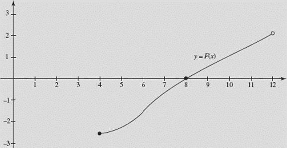
FIGURE N6–22c
Chapter Summary
In this chapter, we have reviewed definite integrals, starting with the Fundamental Theorem of Calculus. We’ve looked at techniques for evaluating definite integrals algebraically, numerically, and graphically. We’ve reviewed Riemann sums, including the left, right, and midpoint approximations as well as the trapezoid rule. We have also looked at the average value of a function.
This chapter also reviewed integrals based on parametrically defined functions, a BC Calculus topic.