Calculus AB and Calculus BC

CHAPTER 7 Applications of Integration to Geometry

D. IMPROPER INTEGRALS

There are two classes of improper integrals:

(1) those in which at least one of the limits of integration is infinite (the interval is not bounded); and

(2) those of the type where f (x) has a point of discontinuity (becoming infinite) at x = c, a c b (the function is not bounded).

Illustrations of improper integrals of class (1) are:

The following improper integrals are of class (2):

Sometimes an improper integral belongs to both classes. Consider, for example,

In each case, the interval is not bounded and the integrand fails to exist at some point on the interval of integration.

Note, however, that each integral of the following set is proper:

The integrand, in every example above, is defined at each number on the interval of integration.

Improper integrals of class (1), where the interval is not bounded, are handled as limits:

where f is continuous on [a,b]. If the limit on the right exists, the improper integral on the left is said to converge to this limit; if the limit on the right fails to exist, we say that the improper integral diverges (or is meaningless).

The evaluation of improper integrals of class (1) is illustrated in Examples 17–23.

EXAMPLE 17

Find

SOLUTION: The given integral thus converges to 1. In Figure N7–22 we interpret as the area above the x-axis, under the curve of y = 3, and bounded at the left by the vertical line x = 1.

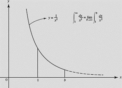
FIGURE N7–22

BC ONLY

EXAMPLE 18

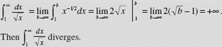
It can be proved that converges if p > 1 but diverges if p 1. Figure N7–23 gives a geometric interpretation in terms of area of Only the first-quadrant area under bounded at the left by x = 1 exists. Note that

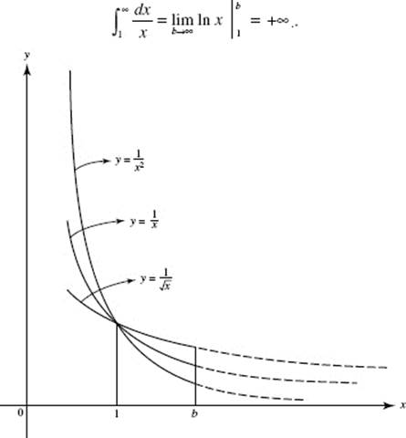
FIGURE N7–23

EXAMPLE 19

EXAMPLE 20

BC ONLY

EXAMPLE 21

EXAMPLE 22

Thus, this improper integral diverges.

EXAMPLE 23

Since this limit does not exist (sin b takes on values between −1 and 1 as b → ∞), it follows that the given integral diverges.

Note, however, that it does not become infinite; rather, it diverges by oscillation.

Improper integrals of class (2), where the function has an infinite discontinuity, are handled as follows.

To investigate where f becomes infinite at x = a, we define to be The given integral then converges or diverges according to whether the limit does or does not exist. If f has its discontinuity at b, we define to be again, the given integral converges or diverges as the limit does or does not exist. When, finally, the integrand has a discontinuity at an interior point c on the interval of integration (a < c < b), we let

Now the improper integral converges only if both of the limits exist. If either limit does not exist, the improper integral diverges.

The evaluation of improper integrals of class (2) is illustrated in Examples 24–31.

BC ONLY

EXAMPLE 24

Find

SOLUTION:

In Figure N7–24 we interpret this integral as the first-quadrant area under and to the left of x = 1.

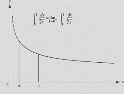
FIGURE N7–24

EXAMPLE 25

Does converge or diverge?

SOLUTION:

Therefore, this integral diverges.

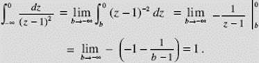
It can be shown that (a > 0) converges if p < 1 but diverges if p 1. Figure N7–25 shows an interpretation of in terms of areas where 1, and 3. Only the first-quadrant area under to the left of x = 1 exists.

Note that

BC ONLY

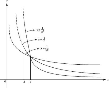
FIGURE N7–25

EXAMPLE 26

EXAMPLE 27

This integral diverges.

EXAMPLE 28

BC ONLY

EXAMPLE 29

Neither limit exists; the integral diverges.

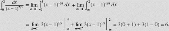
NOTE: This example demonstrates how careful one must be to notice a discontinuity at an interior point. If it were overlooked, one might proceed as follows:

Since this integrand is positive except at zero, the result obtained is clearly meaningless. Figure N7–26 shows the impossibility of this answer.

FIGURE N7–26

THE COMPARISON TEST

We can often determine whether an improper integral converges or diverges by comparing it to a known integral on the same interval. This method is especially helpful when it is not easy to actually evaluate the appropriate limit by finding an antiderivative for the integrand. There are two cases.

(1) Convergence. If on the interval of integration f (x) ≤ g(x) and is known to converge, then also converges. For example, consider We know that converges. Since the improper integral must also converge.

(2) Divergence. If on the interval of integration f (x) ≥ g(x) and is known to diverge, then also diverges. For example, consider We know that diverges. Since sec x ≥ 1, it follows that hence the improper integral must also diverge.

BC ONLY

EXAMPLE 30

Determine whether or not converges.

SOLUTION: Although there is no elementary function whose derivative is e^−x2, we can still show that the given improper integral converges. Note, first, that if x 1 then x² x, so that −x² −x and e^−x2 e^−x. Furthermore,

Since converges and dx converges by the Comparison Test.

EXAMPLE 31

Show that converges.

SOLUTION:

we will use the Comparison Test to show that both of these integrals converge. Since if 0 < x 1, then x + x⁴ > x and it follows that

We know that converges; hence must converge.

Further, if x 1 then x + x⁴ x⁴ and so

We know that converges, hence also converges.

Thus the given integral, converges.

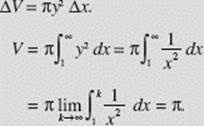
NOTE: Examples 32 and 33 involve finding the volumes of solids. Both lead to improper integrals.

BC ONLY

EXAMPLE 32

Find the volume, if it exists, of the solid generated by rotating the region in the first quadrant bounded above by at the left by x = 1, and below by y = 0, about the x-axis.

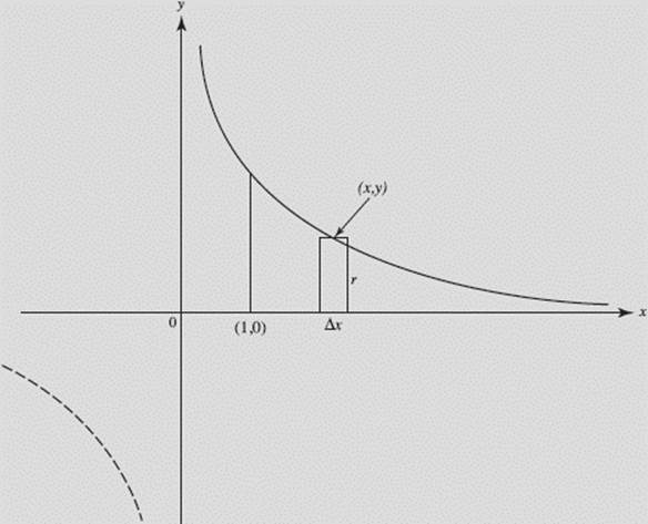
FIGURE N7–27

SOLUTION:

About the x-axis.

Disk.

BC ONLY

EXAMPLE 33‡

Find the volume, if it exists, of the solid generated by rotating the region in the first quadrant bounded above by at the left by x = 1, and below by y = 0, about the y-axis.

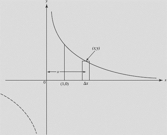
FIGURE N7–28

SOLUTION:

About the y-axis.

Shell.

ΔV = 2πxy Δx = 2π Δx.

Note that diverges to infinity.

Chapter Summary

In this chapter, we have reviewed how to find areas and volumes using definite integrals. We’ve looked at area under a curve and between two curves. We’ve reviewed volumes of solids with known cross sections, and the methods of disks and washers for finding volumes of solids of revolution.

For BC Calculus students, we’ve applied these techniques to parametrically defined functions and polar curves and added methods for finding lengths of arc. We’ve also looked at improper integrals and tests for determining convergence and divergence.

^‡No question requiring the use of shells will appear on the AP exam.