Burn Math Class: And Reinvent Mathematics for Yourself (2016)

6. Two in One

6.4. The Second Cloud

We’ve conquered curviness in two different domains already — first steepness, now area — but we still don’t know how to compute the lengths of curvy things. It’s worthwhile at this point to look at the collected memoirs of our journey, and see what has helped us in the past.

In the domain of steepness, we conquered curviness by zooming in infinitely far on a curvy machine m (at a point x whose value we chose to remain agnostic about) and computing its steepness as if it were a straight line.

In the domain of area, we conquered curviness by realizing that the tiny area under a machine’s graph at each point x can be thought of as an infinitely thin rectangle, with area m(x)dx. Then we just imagined adding up all the tiny areas. We had no idea how to do this at first, but we came up with a name for the unknown answer: . Once we discovered the fundamental hammer, we found that our new ∫ idea was just our old derivative idea in reverse.

Now what? We’ve got enough experience with our magnifying glass that it shouldn’t be too difficult to at least write down an expression for the lengths of curvy things. Whether or not we can actually compute the lengths of curvy things in any particular case is a different story, just as it was in the case of area. Our experience with the magnifying glass so far suggests that we start with a machine m, and then imagine zooming in infinitely far on some point of its graph, remaining agnostic about which particular point we’re zooming in on. Then, as always, let’s look at some other point that’s infinitely close to the first one. See Figure 6.6 for a picture of this situation.

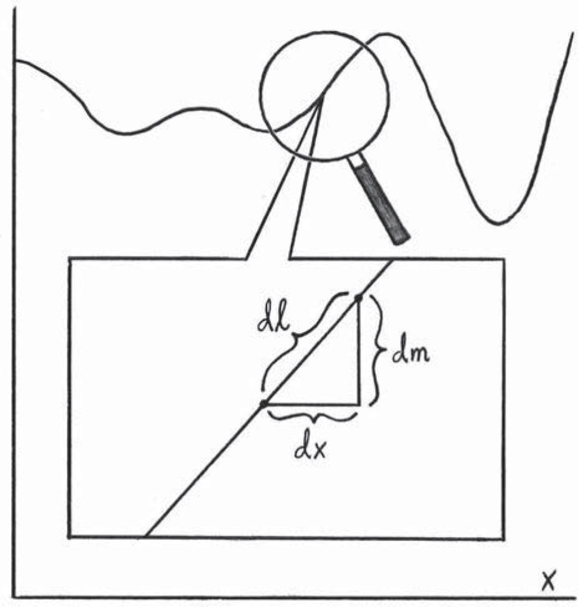
Figure 6.6: Trying to think of a way to compute the lengths of curvy things. The zooming in idea has worked in the past, so let’s try it again. We zoom in infinitely far on the graph of some machine m at some point x, and the curve looks straight. Then we can use the formula for shortcut distances to compute the tiny length dℓ. Then I guess we just add up all the pieces. Wait, is that it?

Once we’ve zoomed in, the problem becomes much less intimidating. We’ve got two points whose horizontal distance apart we’re calling dx, and whose vertical distance apart we’re calling dm. As always, dm is just an abbreviation for m(x + dx) − m(x), but we won’t need to unwrap this abbreviation for our current purposes. Let’s write dℓ as an abbreviation for the actual distance between the two points — that is, the distance we’d experience if we were walking along the graph. Since zooming in turned the curvy thing into an infinitely small straight thing, we can use the formula for shortcut distances to write this:

(dℓ)² = (dx)² + (dm)²

or equivalently, . Whatever the total length of our curvy thing happens to be, it should be whatever we would get if we could somehow add up all the infinitely small pieces dℓ.

What do we mean by the “total length” of a curvy thing? The curve might go on forever, in which case the answer would be infinity, but that’s not quite the question we meant to ask. We really want to talk about the length of m’s graph between any two points x = a and x = b. So, to summarize this paragraph in symbols, it should be the case that:

Okay. . . We haven’t seen anything like this before. We’re only used to expressions involving the ∫ symbol that look like this:

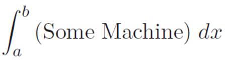
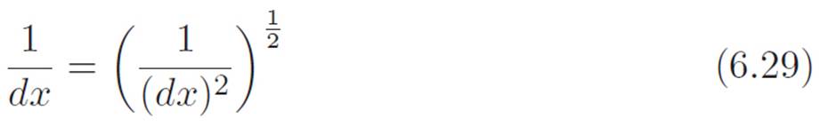
So let’s try to force the piece in equation 6.27 to look like (Some Machine) dx. We can lie and correct to get 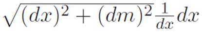. The dx piece on the far right is what we wanted, but the leftovers are pretty ugly. Let’s try to bring the 1/(dx) inside the rest of the leftovers. The square root symbol makes it harder to remember what we’re allowed to do, so let’s turn the square root symbol into a power. Because of the way we invented powers, we know that we can merge two things if they have the same power, like this:

So if we want to move the inside the confusing leftovers, this suggests that we should lie and correct yet again, to write the in this funny sort of way:

If we do that, then we can pick up where we left off and write the following. Don’t be scared by the mountain of symbols below this! It looks like there are a ton of steps in the derivation below, but most of them could probably be skipped. I’m showing more steps because I really like this derivation, and I want it to be as easy as possible to understand each step. But each step is really simple. Ready? Here we go:

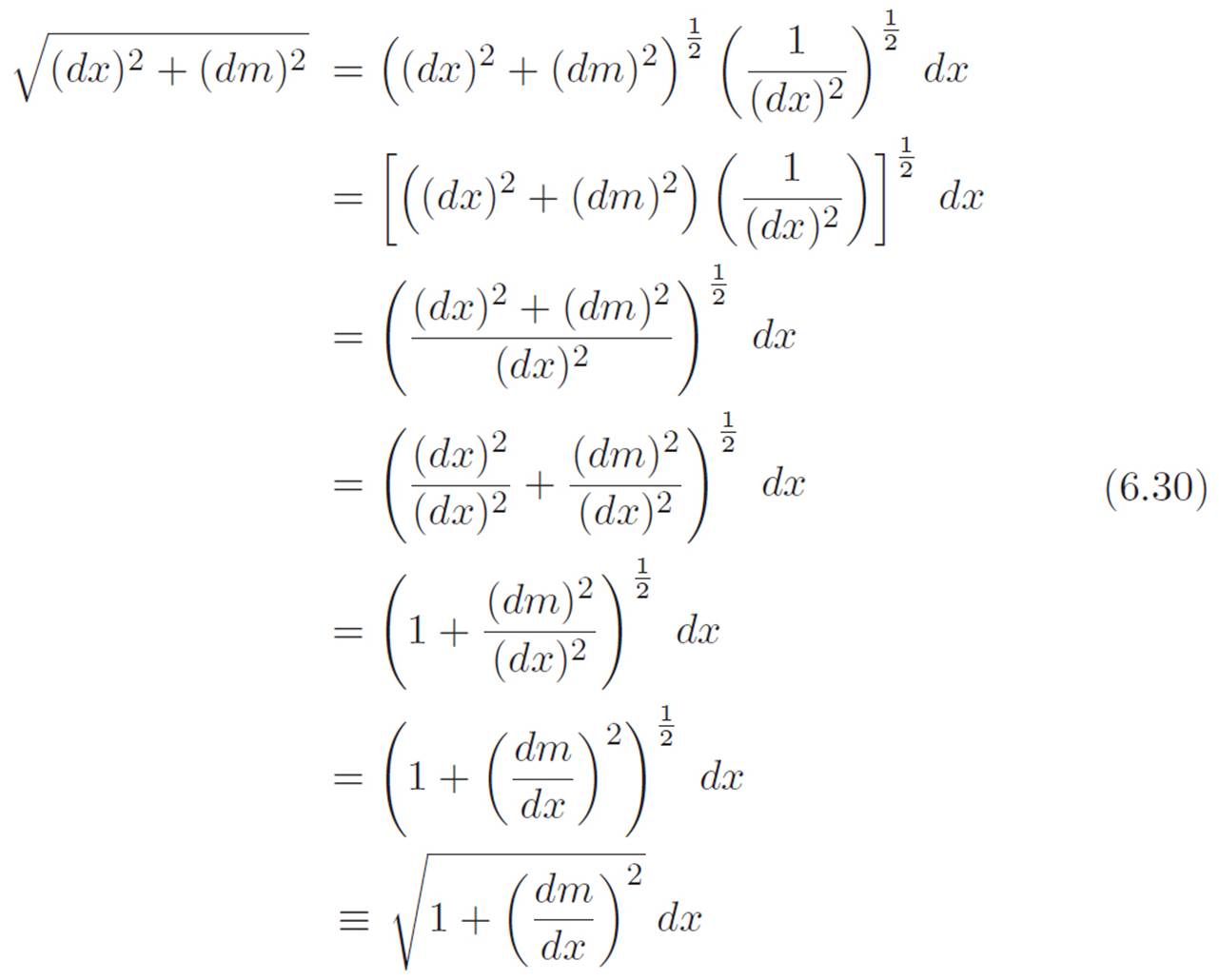
Now for the fun part. We can use this insight to write equation 6.27 in a much less confusing way. Simply throwing the equation we just derived into 6.27, we discover that the total length of any curvy thing m can be written like this:

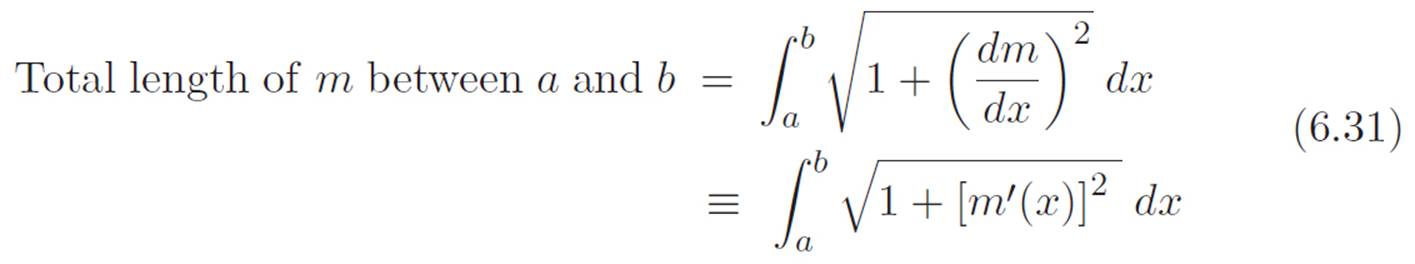
Beautiful! In the first part of this chapter, we found out that our new ∫ idea was just the opposite of our old derivative idea, so in that sense we got two ideas in one. Just now, we had a newer idea of computing the length of a curvy thing by zooming in until it looks straight, measuring the tiny piece of length down there at the microscopic level, and then adding up the tiny lengths. Surprisingly, we’ve now discovered that this idea is really the same idea as the ∫ thing, which was just the opposite of the derivative. Everything hangs together so nicely, and in a way that is so much prettier than we had any reason to expect! Equation 6.31 summarizes everything we did in this section, and as complicated as it looks, it is just saying something like this:

Question: Hey, I’ve got a curvy thing m(x). How do I compute its length?

Answer: I don’t know, but it’s the same as the area under

Question: Does that make the length easier to compute?

Answer: Maybe for certain m’s. I don’t know. Leave me alone.