Burn Math Class: And Reinvent Mathematics for Yourself (2016)

N. New Is Old

N.2. The Notational Minefield of Multivariable Calculus

To most outsiders, modern mathematics is unknown territory. Its borders are protected by dense thickets of technical terms; its landscapes are a mass of indecipherable equations and incomprehensible concepts. Few realize that the world of modern mathematics is rich with vivid images and provocative ideas.

—Ivars Peterson, The Mathematical Tourist

N.2.1Simple Generalizations and Difficult Abbreviations

In the above dialogue, we “invented” multivariable calculus. For example, we looked at machines that eat one number and spit out two numbers, such as m(x) ≡ (f(x), g(x)). Textbooks call these “vector-valued functions,” meaning that they eat a number and spit out a vector. “Vector” means basically the same thing as “list” (for our purposes), and in the remainder of the book, we’ll use the two terms interchangeably. Notice that our pre-mathematical arguments in this interlude apply equally when the vectors have n slots. That is, we can simply dictate that we want lists with n slots to behave like this:

(x₁, x₂, . . . , x_n) + (y₁, y₂, . . . , y_n) = (x₁ + y₁, x₂ + y₂, . . . , x_n + y_n)

c · (x₁, x₂, . . . , x_n) = (cx₁, cx₂, . . . , cx_n)

Again, we’re doing the simplest thing we can think of. These definitions allow us to show, in exactly the same manner as we did in the above dialogue, that the derivative of a “one in, n out” machine such as

m(x) ≡ (f₁(x), f₂(x), . . . , f_n(x))

is the simplest thing we could possibly hope for, namely

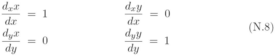
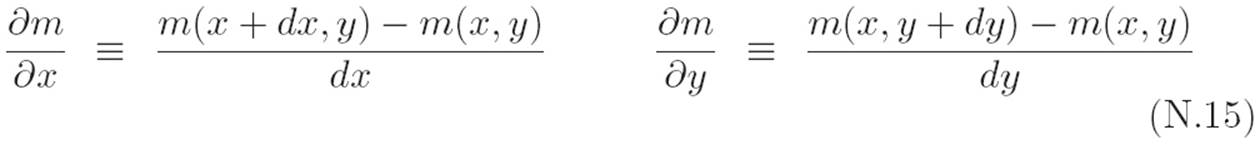
Similarly, for machines that eat two numbers and spit out one number, which we abbreviated as m(x, y), we again found a direct familiarity with single-variable calculus. We preserved the familiarity by simply defining two different derivatives: one for each input. That is, we had a derivative with respect to x (which treated y as a constant), and a derivative with respect to y (which treated x as a constant). We decided to write these as:

Textbooks call these “partial derivatives.” They would call the one on the left “the partial derivative of m with respect to x,” and they would call the one on the right “the partial derivative of m with respect to y.” However, there’s nothing “partial” about partial derivatives: they are computed using the exact same operations as the familiar derivative from Chapter 2. Notice that since we can change x without changing y (and vice versa) we can write expressions like

Again, there’s nothing special about the fact that m(x, y) has only two slots. We can make exactly analogous definitions and arguments when there are n slots. If we define m to be a machine that eats n numbers and spits out one number, which we can write as

then we’ve got n slots, so there are n different derivatives: one for x₁, one for x₂, and so on, up to x_n. Just like before, we can define the derivative this way:

where we’re choosing to write d_i instead of d_xi, because the latter has a subscript on a subscript, which is a bit of a mess. Although the above equation may look scary enough to raise your blood pressure, it’s saying something extremely simple: the derivative of an “n in, one out” machine with respect to some variable x_i is exactly the same thing it has always been. We simply ignore everything that isn’t x_i, and do single-variable calculus thinking of x_i as the only variable. See how this is nothing new? We can clean up the above notation a bit by choosing some simpler abbreviations, which we will do in the next section.

N.2.2Simple Ideas That Resist Simple Expression

I would argue that nearly all of the confusion about multivariable calculus comes from confusions about notation, and in this section we will explore some of the difficulties that arise in attempting to come up with good abbreviations in our new multivariable world.

In single-variable calculus, we’ve kept two notations for the derivative around throughout the book: m′(x) and . The same phenomenon that led us to do so appears in multivariable calculus with even greater force: the ideas themselves seem to resist being clearly expressed by any single set of abbreviations. As before, this leaves us with two options. The first option is to simply decide on one set of abbreviations with which to express all the ideas of multivariable calculus, in which case many conceptually simple expressions will appear hairy and counterintuitive. The second option is to switch notation at will, using whichever is appropriate for the problem at hand. This also has downsides, since there are then multiple symbolic languages floating around. In this chapter, we will err in favor of the latter, but we’ll try to remind ourselves of what the different notations mean whenever we need to switch.

N.2.3Coordinates: (Can’t live with)(1, out)(them)

We will begin by attempting to invent some abbreviations that let us write equation N.10 in a simpler-looking way. To begin, let’s write v as an abbreviation for the machine’s input, so

v ≡ (x₁, x₂, . . . , x_n)

is a list of all n variables. Textbooks use the word “vector” to describe these things, hence the v. The word “vector” may sound bizarre and archaic, but it’s kind of fun to say, so let’s keep it around. We’re writing the vector v in boldface to remind ourselves that it is a different type of object than a number. Let’s write dv_i as an abbreviation for the vector that has zero in every slot except the i^th slot, in which it contains the infinitely small number dx_i. That is:

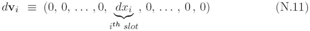
With these conventions, we can rewrite the messy definition in equation N.10 like this:

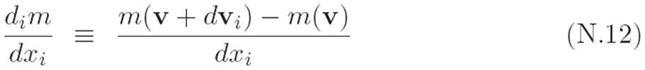
That’s a bit nicer, and it certainly takes up a lot less space, but this notation can be confusing for a completely new reason. Why? Well, glancing casually at the above equation makes it seem as if derivatives in this new multivariable world are something different from what they were in the single-variable world. Why? In the above equation, the tiny object on the top looks like dv_i, which is a “tiny vector,” whereas the tiny object on the bottom looks like dx_i, a “tiny number.” That is, it seems as if there are two different types of tiny thing in this equation: a tiny number and a tiny vector. But notice that this is the fault of the new abbreviations we chose in an attempt to make equation N.10 look less scary.

Equation N.10, despite its drawbacks, made it more clear that there is really only one type of tiny thing on the top and the bottom. And that in turn makes it clear that the derivative has the same interpretation it has always had. That is, we’ve always been able to talk about derivatives like this:

1.We start with a machine m that we feed some stuff s. It spits out m(s).

2.We make a tiny change in the stuff we’re feeding the machine, changing it from s to s + ds. This changes the output from m(s) to m(s + ds).

3.We can abbreviate the change in output as something like dm ≡ m(s + ds) − m(s). If we’ve got more than one variable, we may want to modify our abbreviations to remind ourselves what we’re changing.

4.Whether the stuff s is a number, a vector, or an entire machine, the derivative is the same concept. The derivative of m is defined to be the tiny change in output dm, divided by the tiny change in the input ds.

So the two abbreviations in N.10 and N.12 have different costs and benefits. We’re in an odd Catch-22 situation. As we’ll see soon, the Catch-22 is more general than this example.

N.2.4To ∂ or Not to ∂? Abbreviations Affecting Arguments

The next stop on our tour of the confusing notation in multivariable calculus is the alien symbol ∂. Earlier, I mentioned that the textbooks use the term “partial derivative” to refer to expressions like these:

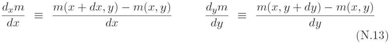
Examining the standard notation for this concept will reveal another Catch-22. Here’s the issue: in the two expressions above, you might notice that writing d_x and d_y is redundant. You might then think that if we simply wrote

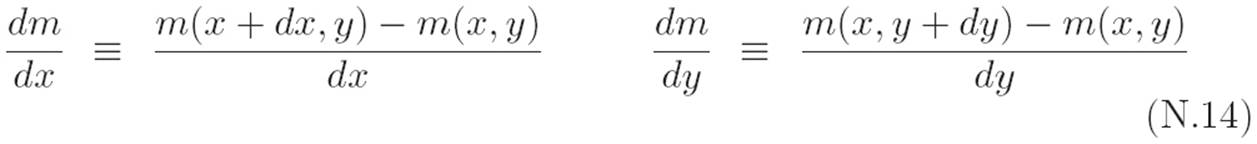
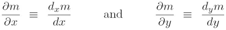
then there would be no confusion, because the dx and dy on the bottom of each expression remind us in which of m’s slots we’re making a tiny change: in the left equation it’s the x slot, and in the right equation it’s the y slot. That’s certainly true. The subscripts on d_x and d_y are redundant when they show up in derivatives, as they do in equation N.13. So why did we introduce the subscripts in the first place? Well, we originally introduced the notation d_xm and d_ym because the two different occurrences of dm in equation N.14 actually refer to different things, as you can see simply by comparing the top right sides of both equalities: on the left we’re changing the first slot, and on the right we’re changing the second slot. If we’re only ever dealing with derivatives, then there’s no reason to write d_xm and d_ym. We can simply look at the bottom of the derivative to see what variable we’re making a tiny change to. Most textbooks run with this line of thinking in choosing their notation, and write the following instead of equation N.13:

So comparing our notation and theirs, we’ve got

This different way of writing things has its own set of costs and benefits. On the one hand, it’s a lot prettier than the notation I’m using, and it avoids the subscripts x and y, which are unnecessary when we’re talking about derivatives themselves. On the negative side, this ∂ notation makes it much harder to make simple infinitesimal arguments. In the next few paragraphs, we’ll explain why by examining a scary-looking equation that hides a simple idea. In every multivariable calculus book you’ll find the equation

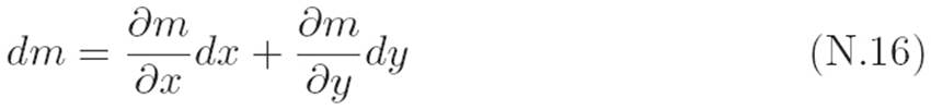
We’ll derive this equation for ourselves very soon, but for the moment, just notice how confusing it looks! This awful equation contains six different symbols that look like infinitely small quantities: dm, ∂m, dy, ∂y, dx, and ∂x. Notice that equation N.16 doesn’t really seem to have anything we can cancel to make it simpler. The crazy ∂x thing looks different from the more familiar dx thing, so it doesn’t feel like we can cancel the ∂x on the bottom against the dx. Same deal for the y’s; cancellation seems illegal, since the symbols look different.

Now, even though we haven’t derived it yet, I can’t resist telling you the ridiculous secret of equation N.16. Here it is: interpreted properly, the ∂x and the dx piece are actually the same thing! Same for the pieces ∂y and dy. As if that weren’t confusing enough, we can then use this fact to get something even worse. Canceling the ∂x against the dx, and doing the same for ∂y and dy, we get this bizarre nonsense:

As we’ll see in a few pages, this equation is actually correct. However, ∂m + ∂m is not equal to 2∂m! No, the laws of arithmetic have not broken down. Rather, in a monumental feat of confusing notation, the two different ∂m pieces in the above equation actually refer to two different things! They refer to what we have been calling d_xm and d_ym, and it was precisely the earlier choice to ignore the (then redundant) subscripts that leads to all of these notational headaches down the road.

Why would anyone use notation in which a single symbol ∂m refers to two different things (d_xm and d_ym) while simultaneously using two different symbols (∂x and dx) to refer to the same thing?! The reason isn’t completely crazy. It’s because the standard textbooks usually don’t use infinitesimal arguments. Given the way all these ideas are usually formalized, most textbooks end up with a number system in which infinitesimals don’t make sense, though derivatives do. But for us, it was clearly beneficial to distinguish between d_xm and d_ym because they’re not the same thing!Textbooks usually neglect the subscripts, and their choice makes sense too: if we’re only talking about derivatives and not the infinitesimals themselves, then the subscripts in d_xm and d_ym are always redundant.

In summary, when using the ∂ notation, we lose one of the best things about the d notation from single-variable calculus: the ability to manipulate infinitesimals just like numbers, canceling them and rearranging their order to derive things that would have been much more difficult to derive otherwise.