Burn Math Class: And Reinvent Mathematics for Yourself (2016)

The Infinite Beauty of the Infinite Wilderness

2. Crossing the Rubicon

.2.1Building a Dictionary for Our Analogy

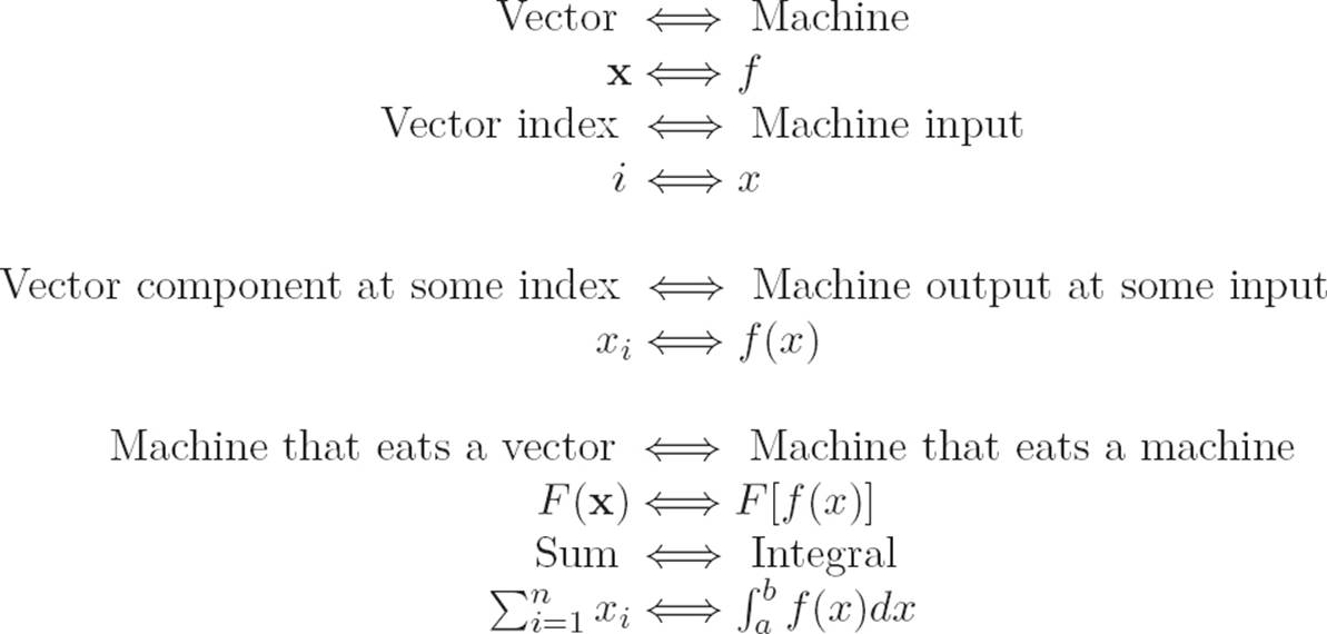
So, having decided to take the analogy between machines and vectors seriously, let’s make this analogy a bit more precise by building a dictionary. This will let us more easily translate back and forth between sentences about vectors and sentences about machines, as well as help us to figure out how we might do calculus in this new infinite-dimensional world. The box below is our dictionary, and each “definition” consists of two lines. The first line of each pair is a description of a particular part of the vector/machine analogy in words, while the second line says the same thing in symbols. The symbol “⇔” means something like “the things on my left and right sides are partners under the vector/machine analogy.” This dictionary is by no means exhaustive; we will notice further ways in which machines and vectors can be unified in the rest of this chapter. However, the dictionary contains a complete description of our thoughts, to this point, about how machines and vectors can be viewed as two specific examples of a more general concept. Ready, set, dictionary!

How the Dictionary Works

Thing about vectors (in words) ⇔ Thing about machines (in words)

Thing about vectors (in symbols) ⇔ Thing about machines (in symbols)

The Dictionary

.2.2Mathematical Cannibalism

By taking seriously the analogy between machines and vectors, we built the above dictionary, which lets us translate from statements about vectors to statements about machines. However, in doing so we wrote down a bunch of symbols that we’re not too familiar with, like F[f(x)].¹ We should stop and ask exactly what kind of objects we’re examining. Much of multivariable calculus consisted of examining machines that eat a vector x and spit out a number F(x). Therefore, taking the vector/machine analogy literally suggests that in the calculus of variations, we are examining machines that eat an entire machine f(x) and spit out a number F[f(x)]. Such cannibalistic machines are usually called “functionals,” and as it turns out, we have met several functionals already, although we did not necessarily think of them in this way at the time. For example, the integral

As a note of clarification, the reason we are using square brackets in writing F[f(x)] is because (i) the notation F(f(x)) is a bit cluttered with parentheses, and (ii) writing F(f(x)) might make it seem as if the machines f and F occupied the same level of abstraction. Although they are both machines, and although the square brackets in F[f(x)] serve exactly the same purpose as normal parentheses would, the slight difference in notation does serve to remind us that f is a machine that eats a number and spits out a number, while F is a machine that eats an entire machine and spits out a number. This is an important distinction: though normal functions such as f can appear in terms such as f(g(x)), the machine f is still simply eating a number, g’s output at input x, while F is genuinely eating an entire machine. F is a cannibal; f is not.

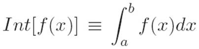
can be thought of as a machine in its own right. That is, a “large machine” that eats an entire machine f(x) and spits out a number: the area under f(x)’s graph between x = a and x = b. Feeding different machines to the cannibalistic machine Int gives us different numbers.

Another example that we’ve already encountered is the so-called “arclength functional.” Toward the end of Chapter 6, we showed that the integral

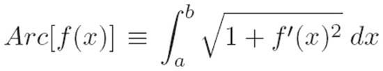
can be thought of as a large machine that eats an entire machine f(x) and spits out a number: the length of f(x)’s graph between x = a and x = b.

Yet another example of a functional is what is often called the “norm” of a machine f. “Norm” is just a fancy word for the “length” of f when interpreted as a vector in an infinite-dimensional space. This interpretation of length has nothing to do with the arclength interpretation above. Rather, it comes from generalizing the familiar concept of a vector’s length — taking inspiration from the formula for shortcut distances — to define a concept of “length” in infinitely-many dimensions. Since we haven’t yet seen this particular kind of cannibalistic machine, it will be useful to take a few minutes to show where the idea comes from, in order to get a better feeling for the type of reasoning we’ll be using in this new infinite-dimensional world.

.2.3Characterizing Length in the Infinite Wilderness

In Interlude 1, we invented the formula for shortcut distances, also known as the Pythagorean theorem. First, notice that we can interpret this formula as a fact about vectors in two dimensions. The components x and y of a vector v ≡ (x, y) are just lengths, and they lie in two perpendicular directions, so the length of this vector should be

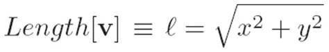
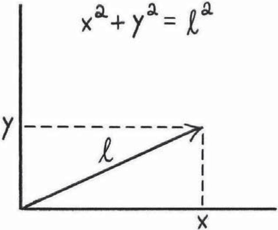
Figure .1: The formula for shortcut distances tells us that the length of a vector v ≡ (x, y) is . This will serve as our inspiration for defining length in the infinite wilderness.

Now, the question arises of whether a similar formula holds in three dimensions, four dimensions, and so on. Since the length of a vector in two dimensions involves a bunch of 2’s (namely, a sum of the components each raised to a power of 2, and with a over the whole thing), we might guess that this relationship between the dimension in which the vector lives (namely, 2) and the powers that show up in the formula (also 2) is not merely a coincidence. This might lead us to guess that the formula for the length of a vector v ≡ (x, y, z) in three dimensions should be

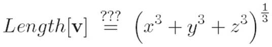
However, while we could certainly choose to measure length this way,² it is not up to us to decide this issue, if we want length to have the same meaning as it does in everyday language. While we are free to do, say, and invent whatever we want, length has an independent, everyday meaning that everyone understands without any mathematics, so if we want “length” to mean what we mean in everyday life, then the definition of the length of a vector in three or four or n dimensions is not something that we can simply invent, but rather something that we have to discover. Since the only raw materials we have at present to attack this question come from the two-dimensional formula for shortcut distances, it is worth asking whether we can use this formula to discover the corresponding unknown formula in higher dimensions, and ultimately extend it to our new infinite-dimensional wilderness.

And mathematicians have done so. Such a way of measuring length is known as the “three norm.” While it has no particular connection with three dimensions, it is a perfectly reasonable definition of length, although it does not correspond with what we mean by length in everyday life. Since it does not correspond with our everyday concept of length, it will not concern us here.

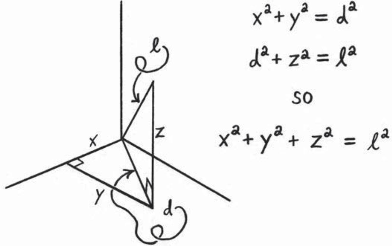
Figure .2: Using the formula for shortcut distances twice lets us build a three-dimensional version of the original formula. It shows us that the length of a vector v ≡ (x, y, z) in three dimensions is .

As Figure .2 shows, it is indeed possible to build a formula for shortcut distances in three dimensions using only the two-dimensional version. This argument demonstrates that

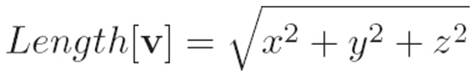
is the length of a vector v ≡ (x, y, z) in three dimensions. Now, by applying the two-dimensional version over and over, we can build an analogous formula for shortcut distances in n dimensions. As expected, it has the same form: the length of a vector x ≡ (x₁, x₂, . . ., x_n) in n dimensions is

Now, if we’re really taking the correspondence between machines and vectors seriously, then we should be able to define the “length” or “size” of a machine by simply interpreting the machine as a vector with infinitely many slots. This would give us a kind of “formula for shortcut distances” in an infinite-dimensional space, and in that sense, it would be a statement about infinite-dimensional geometry. That may sound complicated, but the apparent complexity is mostly the fault of the words we’re using to describe the idea, like “infinite-dimensional space” and such. Despite the sophisticated-sounding language, the underlying idea is extremely simple. We’re really just mindlessly generalizing equation .1 by using our dictionary. That is, all we’re saying is: if we’re thinking of machines as vectors, then equation .1 tells us that the “length” of a machine should be whatever we get from (i) squaring each slot, (ii) adding them all up, and (iii) throwing a square root symbol over the whole thing. That is:

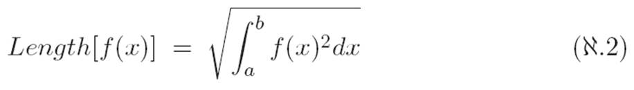
Then, having mindlessly generalized the formula for shortcut distances, we can say all sorts of things that make us sound very smart, like “the length of a function f, interpreted as a vector in an infinite-dimensional space, is simply the square root of the integral of f(x)².” And we know exactly what we mean by sentences of this form, even though we ourselves can’t even begin to picture what we’re saying! Sneaky trick, right? How do we know if this is right? Well, as always, if we want our infinite-dimensional space to behave like the finite-dimensional spaces we’re familiar with, then we can just define length in the infinite wilderness by equation .2. At this point we are engaged not in standard mathematics but rather in pre-mathematics, so the argument above cannot be right or wrong. It is simply using mathematical concepts to make an argument whose apparent merit (or lack thereof) leads us to choose a particular definition of infinite-dimensional length in the first place.

Now that we’ve defined a notion of the “length” of a machine, we can say things like “such and such machine is infinitely small.” That is, now that we can talk about size in the infinite wilderness, we can begin to explore some ideas of how we might invent infinite-dimensional calculus!